Methods of Estimation¶

import matplotlib.pyplot as plt
import numpy as np

Method of moments estimation¶

Want to find a statistic \(T(X_1,...,X_n)\) s.t. \(E_\theta[T(X_1,...,X_n)] = h(\theta)\) where \(h\) has a well-defined inverse. Then, we can set \(T(X_1,...,X_n) = h(\hat\theta)\) s.t. \(\hat\theta = h^{-1}(T)\)

If \(X_1,..., X_n\) indep. and \(E_\theta(X_i) = h(\theta)\), then by substitution principle, we can estimate \(E_\theta(X_i)\) by \(\bar X\) and then \(\bar X = h(\hat\theta)\) and so \(\hat\theta = h^{-1}(\bar X)\)

Example: Exponential Distribution¶

\(X_1,...,X_n\) indep, \(f(x;\lambda) = \lambda \exp(-\lambda x), x\geq 0\), \(\lambda > 0\) is unknown.

Note that for \(r > 0, E_\lambda (X_i^r) = \lambda ^{-r}\Gamma(r+1)\) so that we have MoM estimator

\[n^{-1}\sum^n X_i^r = \frac{\Gamma(r+1)}{\hat\lambda^r}\]

\[\Rightarrow \hat\lambda(r) = \bigg((n\Gamma(r+1)^{-1}\sum^nX_i^r)\bigg)^{-1/r}\]

Using \(r = 1\) gives the best estimation (minimized s.d.)

Example: Gamma Distribution¶

\(X_1,...,X_n\) indep. \(f(x;\lambda, \alpha) = \lambda^a x^{a-1}exp(-\lambda x) \Gamma(a)^{-1}, x\geq 0\). \(\lambda, a > 0\) are unknown. Note that \(E(X_i) = a/\lambda, var(X_i) = a/\lambda^2\), so that MoM gives

\[\bar X = \hat a / \hat \lambda , S^2 = \hat a / \hat \lambda^2\]

\[\Rightarrow \hat a = \bar X^2 / S^2 , \hat \lambda = \bar X / S^2\]

Confidence Interval¶

An interval \(\mathcal I = [l(X_1,...,X_n), u(X_1,...,X_n)]\) is a CI with coverage \(100p\%\) if

\[P[l(X_1,...,X_n)\leq \theta \leq u(X_1,...,X_n)] = p, \forall \theta\in\Theta\]

The pivotal method¶

Is not that often that we can measure such probability directly. One way to work around is to find a r.v. \(g(X_1,...,X_n,\theta)\) whose distribution is independent of \(\theta\) and any other unknown params.

Confidence Interval¶

An interval \(\mathcal I = [l(X_1,...,X_n), u(X_1,...,X_n)]\) is a CI with coverage \(100p\%\) if

\[P[l(X_1,...,X_n)\leq \theta \leq u(X_1,...,X_n)] = p, \forall \theta\in\Theta\]

Example¶

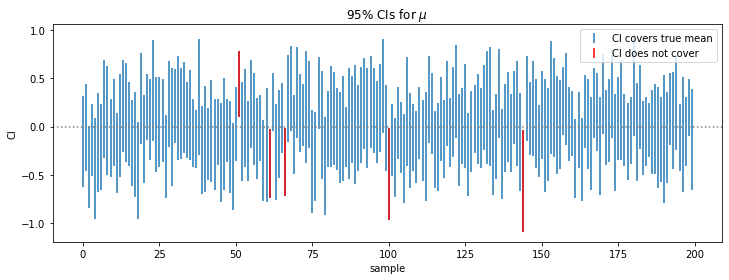
For \(X_1,...,X_{20}\) indep. \(\sim N(\mu, \sigma^2)\), the \(95\%\) CI is \([\bar X\pm -2.093\frac{S}{\sqrt{20}}]\).

The following example is 100 samples of size 20 from \(N(0, 1)\) and we note that \(95\%\) of the samples falls into the confidence interval.

samples = np.random.randn(200, 20)
mean = samples.mean(axis=1)
sd = samples.std(axis=1)
not_in_CI = np.concatenate((np.where(mean + 2.093 * sd / samples.shape[1]**0.5 < 0)[0], 
                            np.where(mean - 2.093 * sd / samples.shape[1]**0.5 > 0)[0]))
plt.figure(figsize=(12, 4))
plt.errorbar(x=np.arange(samples.shape[0]), y=mean, 
             yerr = 2.093 * sd / 20**0.5 , 
             fmt=" ", label="CI covers true mean")
plt.errorbar(x=not_in_CI, y=mean[not_in_CI], 
             yerr = 2.093 * sd[not_in_CI] / 20**0.5 , 
             fmt=" ", color="red", label="CI does not cover")
plt.axhline(0, linestyle=":", color="grey")
plt.xlabel("sample"); plt.ylabel("CI")
plt.title(r"95% CIs for $\mu$"); plt.legend();

The pivotal method¶

Is not that often that we can measure such probability directly. One way to work around is to find a r.v. \(g(X_1,...,X_n,\theta)\) whose distribution is independent of \(\theta\) and any other unknown params.

Maximum Likelihood Estimation¶

Given \((X_1,...,X_n)\) r.v. with joint pdf

\[f(x_1,...,x_n; \theta_1,...,\theta_k)\]

where \(\theta\)'s are unknown parameters.
The likelihood is defined as

\[\mathcal L(\theta_1, ...,\theta_k) = f(x_1,...,x_n; \theta_1,...,\theta_k)\]

note that \(x_1,...,x_n\) are fixed observations

Suppose that for each \(\vec x\), \((T_1(\vec x), ..., T_k(\vec x))\) maximize \(\mathcal L (\Theta)\) . Then maximum likelihood estimators (MLEs) of \(\Theta\) are

\[\hat \theta_j = T_j(X_1,..., X_n), j = 1,..., k\]

Existence and uniqueness¶

MLE is essentially an ad hoc procedure albeit one that works very well in many problems.
MLEs need not be unique, although in most cases, it is unique.
MLEs may not exist, typically when the sample size is too small.

Sufficient Statistic¶

A statistic \(T = (T_1(\vec X), ..., T_m(\vec X))\) is sufficient for \(\theta\) if the conditional distribution of \(\vec X\) given \(T = t\) depends only on \(t\).

Neyman Factorization Theorem¶

\(T\) is sufficient for \(\theta\) IFF

\[f(\vec x;\theta) = g(T(\vec x); \theta) h(\vec x)\]

Observed Fisher Information¶

Given the MLE \(\hat \theta\), the observed Fisher information is

\[\mathcal I(\hat\theta) = -\frac{d^2}{d\theta^2}\ln \mathcal L(\hat\theta)\]

Fisher information is an estimator for standard error, i.e.

\[\hat se(\hat \theta) = \{\mathcal I(\hat\theta)\}^{-1/2}\]

Mathematically, this is the absolute curvature of the log-likelihood function at its maximum. If this is small, then the estimator is more well-defined (hence with smaller estimated s.e.)

Approximate normality of MLEs¶

Theorem For \(X_1,...,X_n\) indep. with pdf \(f\) for some real-valued \(\theta\in \Theta\), if

\(\Theta\) is an open set
\(A = \{x: f(x;\theta)> 0\}\) does not depend on \(\theta\) (true for the exponential families)
\(l(x;\theta)\) is 3-time differentiable w.r.t. \(\theta\) for each \(x\in A\).

Then, with \(\theta_0\) being the true parameter, we have

\[\begin{align*} \sqrt n(\hat\theta_n - \theta_0) &\approx \bigg\{-n^{-1}\sum^n l''(X_i; \theta_0)\bigg\}^{-1}\frac{1}{\sqrt n} \sum^n l'(X_i;\theta_0)\\ &\approx \frac{1}{\sqrt n} \sum^n \frac{l'(X_i; \theta_0)}{\mathcal I(\theta_0)}\\ &\rightarrow^d N(0, \mathcal I(\theta_0)^{-1}) \end{align*}\]

proof. This conclusion follows Taylor expansion

\[0 = \frac{1}{\sqrt n} \sum^n l'(X_i;\theta_0) + \{\sqrt n (\hat \theta_n - \theta_0)\} \frac{\sum^n l''(X_i; \theta_0)}{n} + \sqrt n(\hat\theta_n - \theta_0) \times R_n\]

where \(R_n = \frac{1}{2}(\hat\theta_n - \theta_0) \frac{\sum^nl''(X_i; \theta_n^*)}{n}\) is the Taylor's remainder with \(\theta_n^*\) in between \(\hat\theta_n, \theta_0\) so that

\[\sqrt n (\hat\theta_n - \theta_0) =\bigg\{-n^{-1}\sum^n l''(X_i; \theta_0) - R_n\bigg\}^{-1}\frac{1}{\sqrt n} \sum^n l'(X_i;\theta_0)\]

Then, note that \(\hat\theta_n - \theta_0 \rightarrow ^p 0\) (i.e. \(\hat\theta\)) is a "good" estimator from the assumption, and \(\frac{1}{n}\sum l''(X_i; \theta_n^*)\) is bounded. so that their product,

\[ R_n = \frac{1}{2}(\hat\theta_n - \theta_0) \frac{\sum^nl''(X_i; \theta_n^*)}{n}\rightarrow^p 0\]

Therefore, \(\sqrt{\hat\theta_n - \theta_0}\rightarrow^d (0, \mathcal I(\theta_0)^{-1})\)