Attention Optimizations
KV cache size
| Model | Config | Bytes/token | @128K ctx, batch 1 |
|---|---|---|---|
| Llama-3-70B | 80 layers, 8 KV heads, d=128, bf16 | 320 KiB | 40 GiB |
| Llama-3-8B | 32 layers, 8 KV heads, d=128, bf16 | 128 KiB | 16 GiB |
| Hypothetical full-MHA 70B | 80 layers, 64 KV heads, d=128, bf16 | 2.5 MiB | 320 GiB |
This entire 40GiB size cache
- needs to exist on HBM, limiting the maximum concurrency.
- needs to be loaded in each decode forward pass, limiting the forward pass rooflining.
The optimization directions are
S_prior: Attend to fewer tokens → less compute, and sometimes less cache.S_prior: Replace the cache with a fixed-size state** → linear attention / SSMs.n_kv_headsandd_head: A smaller latent KV cache, store fewer K/V vectors per token.n_bytesquantization.
Sliding-window and interleaved local/global
Sliding window attention only keeps the most recent \(W\) KV cache. A pure-SWA model cannot do retrieval beyond w × n_layers in principle, and far worse in practice. Therefore, a naturally way is to interleave SWA layers with global attention layers.
Another note is that SWA is different from a max context length = W attention: RoPE will use the token's real position.
- Mistral 7B1 — SWA with window 4096 in every layer. Cache is capped at the window size (rolling buffer), so cache is
O(w), notO(L). Notably, later Mistral models dropped it. - Gemma 2 / 323 — interleaved local:global, 1 global layer per 5 local in Gemma 3. A few global layers preserve long-range retrieval capability, while most layers keep an O(w) cache.
- gpt-oss4 same alternating local/global idea by 1:1 ratio.
Attention sinks
StreamingLLM5 found that if you naively slide the window and drop the first few tokens, perplexity explodes. Keeping just the first ~4 tokens ("attention sinks") plus a rolling window restores it. Explanation: softmax must sum to 1, so heads that want to attend to nothing dump probability mass onto the earliest tokens, which are visible to every query.
Modern models sometimes carry an explicit learned sink logit instead (gpt-oss4, others), which makes them more robust to windowing.
Query-aware retrieval
The cache stays whole but each decode step computes a cheap per-page summary statistic, takes the top-k pages by that statistic, and attends only over those. Note that it does not reduce HBM pressure on its own, but memory loading.
Early explorations are on the serving stack only: HiSparse6 — full KV in host memory, fixed-size GPU cache, hit-detection + LRU + prefetch fused inside the decode CUDA graph. Bit-identical outputs, up to 4.7× throughput. Merged into SGLang.
More recent models moved to native sparse attention. The model's own attention is shaped around the slice it will actually read, hence hold quality at far smaller k than inference-time chosen top-k.
DSA: DeepSeek Sparse Attention 7
DSA+MLA needs to work together: DSA is only affordable because MLA already collapsed K and V into a single vector per token.
DSA uses a top-k indexer to reduce per-head cache computations (but this won't reduce HBM pressure).
MLA8 reduces KV cache from 2 * n_kv_heads * d_head to a single d_latent + RoPE_coef = 512 + 64 = 576 (shapes as in DeepSeek-V39). However, for each head in the SDPA compute, we need to expand the latent cache them back via a linear layer. Therefore, if we need to compute over the full context length, the computation is much larger.
Computation Path
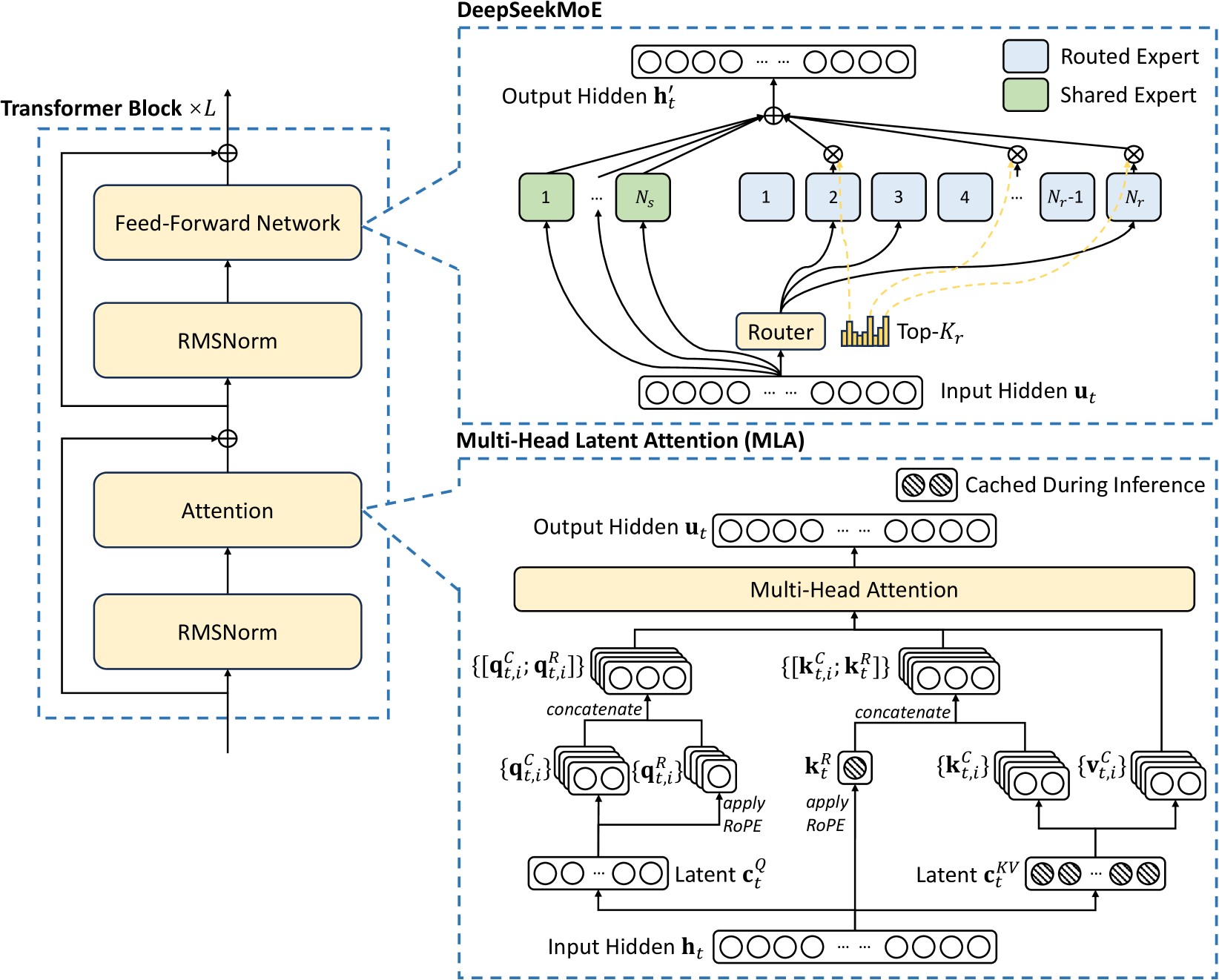
# input: h = (1, 7168)
# W_* are the linear layers

# Query path
c_Q = q_norm(W_qa(h)) # latent q (1, 1536)
q = W_qb(c_Q).view(n_q_heads, qk_head_dim)
q_nope, q_pe = torch.split(q, (qk_nope_dim, qk_rope_dim)) # Q nope + Q RoPE (1, 128, 128 + 64)
q_pe = RoPE(q_pe, freqs_cis)
q = torch.cat(q_nope, q_pe) # Q (1, 128, 192)

# new latent KV
c_KV = W_kv(h) # latent KV (1, 512)
k_pe = RoPE(W_kr(h)) # K RoPE (1, 64)

# --- Cache size (S_prior, 576) ---
update_cache(torch.cat(c_KV, k_pe))
# ---------------------------------

# Indexer
q_i = W_qi(c_Q).view(n_heads, qk_head_dim)
q_i_nope, q_i_pe = torch.split(q_i, (indexer_nope_dim, indexer_rope_dim)) # Q nope + Q RoPE for indexer (1, 64, 64 + 64)
q_i_pe = RoPE(q_pe, freqs_cis)
q_i = torch.cat(q_i_nope, q_i_pe) # Q (1, 64, 128)

k_i = k_norm(W_ki(h)) # indexer k (1, 128)
k_i_nope, k_i_pe = torch.split(k_i, (indexer_nope_dim, indexer_rope_dim)) # K nope + K RoPE for indexer (1, 128, 64 + 64)
k_i_pe = RoPE(k_i_pe, freqs_cis)
k_i = torch.cat(k_i_nope, k_i_pe) # Q (1, 128)

# --- Cache indexer size (S_prior, 128) ---
update_cache(k_i)
# ---------------------------------

w = W_m(h) * n_heads ** -0.5 # mixing weight per token per head (1, 64)

# indexer score (1, 64, 1, 128) * (128k, 1, 128, 1) -> (128k, 64)
I = (w * torch.bmm(q_i[:, :, None, :], k_i[:, None, :, None]))[:, : , 0, 0]

indices = topk(I, k=2048) # pick up the top 2048 scores

# retrieve k and v for SDPA
c_prior, k_prior_rope = torch.split(c_cache[indices], (latent_dim, qk_rope_dim)) # (128k, 576) -> (2048, 512 + 64)
kv_prior = W_kv(c_prior).view(k, 2, n_heads, qk_nope_dim) # (2048, 2, 128, 128)
k_prior = torch.cat(kv_prior[:, 0, :, :], k_prior_rope) # (2048, 128, 192)
v_prior = kv_prior[:, 1, :, :] # (2048, 128, 128)

# Now we have the tensors required for SDPA
# q: (1, 128, 192)
# k_prior: (2048, 128, 192)
# v_prior: (2048, 128, 128)
KV Cache Memory Pressure
Per decode step at 128K context, batch 1, bf16 latent (61 layers):
| HBM | Memory loading | |
|---|---|---|
| MLA latent | 128k x 576 × 61 x 2B = 8.57 GiB |
(2k/128k) x 8.57 GiB = 0.13 GiB |
| Indexer keys | 128k x 128 x 61 x 1B = 0.95 GiB |
0.95 GiB |
| DSA total | ≈ 9.52 GiB | ≈ 1.1 GiB |
Computation Considerations
For MLA, effectively we are trading the KV cache memory with a linear projection. Most considerably the W_kv(c_prior) which maps (S_prior, 512) -> (S_prior, 2, 128, 128). Compared with GQA (since in practice we will share KV heads), we are trading this with a memory loading of (S_prior, 2, 8, 128). On top of this, we also use DSA to reduce S_prior from 128k to 2k, with an overhead of indexer cache, some projections, and a topk operator (The topk can be expensive).
Some roofline analysis:
H200 SXM: 4.8 TB/s HBM3e, 989 TFLOP/s bf16 dense, 1979 TFLOP/s fp8 dense. Computational intensity = 206 FLOP/byte (bf16), 412 FLOP/byte (fp8).
Per layer, per decode step, batch 1, S_prior = 2048 selected tokens, 128 query heads, bf16 cache.
"Bytes" counts cache traffic only — weights are handled separately below.
| Path | FLOPs | Bytes | AI (FLOP/B) | Bound | time/layer |
|---|---|---|---|---|---|
| GQA, 8 KV heads | 134 M | 8.39 MB | 16 | memory | 1.75 us |
| MLA | 604 M | 2.36 MB | 256 | compute | 0.61 us |
Note that since GQA is heavily memory bound, MLA's latent projections are almost given "for free", since computation engines are idle.
Another note is that MLA requires larger concurrency: the projection weights is ~33.6 MiB per layer, so the trade-off is (8.39MiB * BSZ) vs (2.36 MiB * BSZ + 33.6 MiB).
Caveats
- A 128k-element top-k per token per layer. This can be very expensive.
- DSA does not applied to prefill. Prefill is still \(O(L^2)\) on the score side.
- Quantization headroom is near zero on the latent.
Linear Attention10
Given \(Q, K, V \in \mathbb{R}^{L \times d}\), write softmax attention as
and view it as a special case of
for any non-negative similarity function \(\text{sim}(\cdot, \cdot)\) between queries and keys.
Having swapped \(\text{exp}(QK^T)\) for \(\phi(Q)\phi(K)^T\). — that is, the similarity metric is induced by applying a feature map \(\phi\) independently to \(Q\) and \(K\).
We can exploit the fact that matrix multiplication is associative to reorder operations:
Recurrent form
Linear attention only needs \(\sum_{i=1}^l \phi(k_i)^T\) and \(\sum_{i=1}^l \phi(k_i)^Tv_i\) which is independent of \(\phi(Q)\) so we can reuse the values computed through step \(l-1\).
Concretely, with \(Z_{l-1} = \sum_{i=1}^{l-1} \phi(k_i)^T\) and \(S_{l-1} = \sum_{i=1}^{l-1} \phi(k_i)^Tv_i\):
For \(o_{l+1}\), set \(S_l = S_{l-1} + \phi(k_l)^Tv_l\) and \(Z_l = Z_{l-1} + \phi(k_l)^T\) and repeat.
This is the recurrent view of linear attention: maintain a constant-size state \(S_l\) and normalizer \(Z_l\), and each decoding step costs \(O(1)\) time and memory. This is formally an RNN with matrix-valued state \(S_l \in \mathbb{R}^{d' \times d}\).
Some work1211 drops the \(Z_l\) normalizer due to numerical instability and observes no problems empirically; taking \(\phi\) to be the identity also works, interestingly. That leaves the clean form
KDA: Kimi Delta Attention13
Kimi Linear13 is a 48B-total / 3B-active MoE at 1M context, built from Kimi Delta Attention (KDA) layers and full MLA layers at 3:1 — every fourth layer is full attention. Reported: 75% KV cache reduction, up to 6× decode throughput at 1M, and better quality than the full-attention baseline on their evals.
KDA replaces the state update with
Per head, with state \(S_t \in \mathbb{R}^{d_v \times d_k}\), key/query \(k_t, q_t \in \mathbb{R}^{d_k}\), value \(v_t \in \mathbb{R}^{d_v}\), channel-wise decay \(a_t \in (0,1)^{d_k}\), and write strength \(\beta_t \in (0,1)\). The \(\alpha_t\) and \(\beta_t\) are the "delta", computed from computed per token from the hidden state via linear layer \(W_\alpha,W_\beta\).
Full KDA Layer
The recurrence above is only the middle of the layer. It consumes \(q_t, k_t, v_t, a_t, \beta_t\), and every one of those is itself produced from the hidden state \(x_t \in \mathbb{R}^{d}\). The full path:
1. Project and locally mix with locally previous states Each of \(q, k, v\) gets a linear projection followed by a short convolution of window \(W = 4\). Per channel \(c\), with its own length-\(W\) kernel \(w^{(c)}\):
Likewise for \(k, v\).
# x: hidden state of token index t (1, H)
# q/k/v_conv_state: (3, W - 1, D)
q_proj = W_q(x) # (1, D)

# W_min: (W, C)
# q_proj and q_conv_state concat to (W, C)
q_mixed = conv1d(torch.cat(q_proj, q_conv_state), W_mix) # mixed and add along token dim (1, C)

q = SiLU(q_mixed).view(1, n_heads, d_head)

# same thing for k, v
k = ...
v = ...

update_conv_state(q, k, v)
2. L2 Normalize keys and queries. \(q_t, k_t \leftarrow q_t/\|q_t\|_2,\; k_t/\|k_t\|_2\) per head, then \(q_t \leftarrow d_k^{-1/2} q_t\). The L2 normalization is what keeps \(\left(I - \beta_t k_t k_t^\top\right)\) a well-behaved (norm \(\le 1\)) projection, so the state can't blow up.
3. Compute the gates. The decay comes from a low-rank bottleneck — \(d \to d_h \to n_h d_k\) — squeezed through a Mamba-style parameterization:
4. Run the recurrence. The state update and \(o_t = S_t q_t\) from above, in one of the three execution modes.
5. Gated normalization and output. A second low-rank projection produces an output gate, applied multiplicatively after an RMSNorm on the head output:
Cache Size Memory Pressure
Per decode step at 1M context, batch 1, Kimi Linear's 27 layers (20 KDA + 7 MLA, n_h = 32,
d_k = d_v = 128, MLA latent 512 + 64 = 576):
| Per layer | HBM | Memory loading | |
|---|---|---|---|
| KDA state (fp32) | 32 × 128 × 128 × 4B = 2 MiB |
× 20 = 40 MiB |
40 MiB |
| KDA conv windows (bf16) | 3 × 4096 × 4 × 2B = 96 KiB |
× 20 = 1.9 MiB |
1.9 MiB |
| MLA latent (bf16) | 1M × 576 × 2B = 1.125 GiB |
× 7 = 7.88 GiB |
7.88 GiB |
| Kimi Linear total | ≈ 7.92 GiB | ≈ 7.92 GiB | |
| all-MLA baseline | 1.125 GiB |
× 27 = 30.4 GiB |
30.4 GiB |
Chunk-wise Form
As we can see, this state update is very friendly for decode pass. All linear transformations. However, we can't parallelize tokens during prefill with this naive implementation.
Consider simple linear attention without delta terms, we still have the plain linear attention form \(S = K^T V \odot M\). So we can partition the sequence into chunks:
- across chunks: recurrent, \(L/C\) sequential steps instead of \(L\).
- within a chunk: quadratic attention, which is fine because \(C^2\) is small and it's one dense matmul.
Note that the causal mask \(M\) will be needed. The history term needs no mask — every token in \(S_{[c]}\) is strictly earlier than every token in the chunk, which is the whole trick. Causality only has to be enforced on the small block.
Delta decay gate
With a per-channel decay the state is no longer a plain sum, but the log gate makes the cumulative decay a cumsum.
# per chunk c, with S carried across chunks
g = g.cumsum(dim=0)                        # (C, d_k)  cumulative log decay
A = tril(beta[:, None] * ((K * exp(g)) @ (K / exp(g)).T), -1)
T = inv(I + A) @ diag(beta)                # (C, C)    forward substitution
W, U = T @ (K * exp(g)), T @ V             # pseudo-keys / pseudo-values
V_hat = U - W @ S                          # subtract what S already predicts

Aqk = tril(pairwise(Q, K, g))              # (C, C)    A_ij = q_i·k_j exp(g_i - g_j)
O = (Q * exp(g)) @ S + Aqk @ V_hat         # history + local
S = diag(exp(g[-1])) @ S + (K * exp(g[-1] - g)).T @ V_hat
-
↩
@article{jiang2023mistral7b, title = {Mistral 7B}, author = {Jiang, Albert Q. and Sablayrolles, Alexandre and Mensch, Arthur and Bamford, Chris and Chaplot, Devendra Singh and de las Casas, Diego and Bressand, Florian and Lengyel, Gianna and Lample, Guillaume and Saulnier, Lucile and others}, journal = {arXiv preprint arXiv:2310.06825}, year = {2023} } -
Gemma 2: Improving Open Language Models at a Practical Size
↩@article{gemmateam2024gemma2, title = {Gemma 2: Improving Open Language Models at a Practical Size}, author = {{Gemma Team} and Riviere, Morgane and Pathak, Shreya and Sessa, Pier Giuseppe and Hardin, Cassidy and Bhupatiraju, Surya and Hussenot, L{\'e}onard and Mesnard, Thomas and Shahriari, Bobak and others}, journal = {arXiv preprint arXiv:2408.00118}, year = {2024} } -
↩
@article{gemmateam2025gemma3, title = {Gemma 3 Technical Report}, author = {{Gemma Team} and Kamath, Aishwarya and Ferret, Johan and Pathak, Shreya and Vieillard, Nino and Merhej, Ramona and Perrin, Sarah and Matejovicova, Tatiana and Ram{\'e}, Alexandre and Rivi{\`e}re, Morgane and others}, journal = {arXiv preprint arXiv:2503.19786}, year = {2025} } -
gpt-oss-120b & gpt-oss-20b Model Card
↩↩@article{openai2025gptoss, title = {gpt-oss-120b \& gpt-oss-20b Model Card}, author = {{OpenAI}}, journal = {arXiv preprint arXiv:2508.10925}, year = {2025} } -
Efficient Streaming Language Models with Attention Sinks
↩@inproceedings{xiao2024streamingllm, title = {Efficient Streaming Language Models with Attention Sinks}, author = {Xiao, Guangxuan and Tian, Yuandong and Chen, Beidi and Han, Song and Lewis, Mike}, booktitle = {International Conference on Learning Representations (ICLR)}, year = {2024} } -
HiSparse: Scaling Sparse-Attention Decoding with Hierarchical KV Cache Management
↩@article{xie2026hisparse, title = {HiSparse: Scaling Sparse-Attention Decoding with Hierarchical KV Cache Management}, author = {Xie, Zhiqiang and Huang, Zhangheng and Huang, Tingwei and Xu, Ziyi and Ma, Ruiyang and Kozyrakis, Christos}, journal = {arXiv preprint arXiv:2608.07009}, year = {2026} } -
DeepSeek-V3.2: Pushing the Frontier of Open Large Language Models — DSA was introduced in the earlier V3.2-Exp release; this is the full technical report.
↩@article{deepseek2025v32, title = {DeepSeek-V3.2: Pushing the Frontier of Open Large Language Models}, author = {{DeepSeek-AI}}, journal = {arXiv preprint arXiv:2512.02556}, year = {2025} } -
DeepSeek-V2: A Strong, Economical, and Efficient Mixture-of-Experts Language Model — introduces MLA.
↩@article{deepseek2024v2, title = {DeepSeek-V2: A Strong, Economical, and Efficient Mixture-of-Experts Language Model}, author = {{DeepSeek-AI}}, journal = {arXiv preprint arXiv:2405.04434}, year = {2024} } -
DeepSeek-V3 Technical Report — source for the MLA shapes used above.
↩@article{deepseek2024v3, title = {DeepSeek-V3 Technical Report}, author = {{DeepSeek-AI}}, journal = {arXiv preprint arXiv:2412.19437}, year = {2024} } -
Transformers are RNNs: Fast Autoregressive Transformers with Linear Attention
↩@inproceedings{katharopoulos2020lineartransformers, title = {Transformers are RNNs: Fast Autoregressive Transformers with Linear Attention}, author = {Katharopoulos, Angelos and Vyas, Apoorv and Pappas, Nikolaos and Fleuret, Fran{\c{c}}ois}, booktitle = {International Conference on Machine Learning (ICML)}, year = {2020} } -
Retentive Network: A Successor to Transformer for Large Language Models
↩@article{sun2023retnet, title = {Retentive Network: A Successor to Transformer for Large Language Models}, author = {Sun, Yutao and Dong, Li and Huang, Shaohan and Ma, Shuming and Xia, Yuqing and Xue, Jilong and Wang, Jianyong and Wei, Furu}, journal = {arXiv preprint arXiv:2307.08621}, year = {2023} } -
Gated Linear Attention Transformers with Hardware-Efficient Training
↩@inproceedings{yang2024gla, title = {Gated Linear Attention Transformers with Hardware-Efficient Training}, author = {Yang, Songlin and Wang, Bailin and Shen, Yikang and Panda, Rameswar and Kim, Yoon}, booktitle = {International Conference on Machine Learning (ICML)}, year = {2024} } -
Kimi Linear: An Expressive, Efficient Attention Architecture
↩↩@article{kimi2025kimilinear, title = {Kimi Linear: An Expressive, Efficient Attention Architecture}, author = {{Kimi Team}}, journal = {arXiv preprint arXiv:2510.26692}, year = {2025} }