Classification Optimization¶

Binary Linear Classification¶

Let the target \(t \in \{0,1\}\) be the binary classification, using a linear function model \(z = \vec w^T \vec x\) with threshold \(I(z \geq 0)\)
where \(\vec x\) is the training data with one more dummy variable \(1\) so that the threshold is always \(0\)

Geometric Picture¶

Given input \(t = \text{NOT } x, x\in\{0,1\}\)

Input space¶

the weights (hypothesis) can be represented by half-spaces

\[H_+ = \{\vec x\mid \vec w^T \vec x \geq 0\}, H_- = \{\vec x\mid \vec w^T \vec x < 0\}\]

The boundary is the decision boundary \(\{\vec x\mid \vec w^T \vec x = 0\}\)

If the training example can be perfectly separated by a linear decision rule, we say the data is linearly separable

weight space¶

each training example \(\vec x\) specifies a half space \(\vec w\) must lie in to be correctly classified: \(w^Tx >0\) if \(t = 1\) The region satisfying all the constraints is the feasible region. The problem is feasible is the region \(\neq \emptyset\), otw infeasible

Note that if training set is separable, we can solve \(\vec w\) using linear programming

Loss Function¶

0-1 Loss¶

Define the 0-1 Loss be

\[\mathcal L_{0-1}(y,t) = \mathbb I(y\neq t)\]

Then, the cost is

\[\mathcal J = \frac{1}{N}\sum^N \mathbb I(y^{(i)}\neq t^{(i)})\]

However, such loss is hard to optimize (NP-hard considering integer programming)

Note that \(\partial_{w_j} \mathcal L_{0-1} = 0\) almost everywhere (since \(\mathcal L\) is a step function w.r.t \(z\))

Surrogate loss function¶

If we treat the model as a linear regression model, then

\[\mathcal L_{SE}(y,t) = \frac{(y-t)^2}{2}\]

However, the loss function will give large loss if the prediction is correct with high confidence.

Logistic Activation Function¶

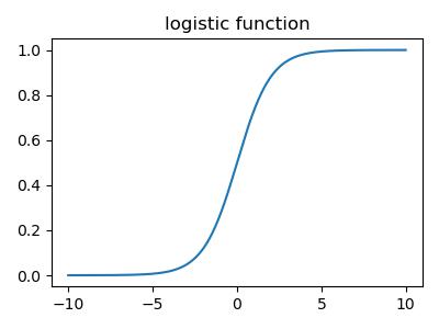
Using logistic function \(\sigma(z) = (1+e^{-z})^{-1}\) to transform \(z = \vec w^T\vec x + b\).

\[\mathcal L_{SE}(y,t) = \frac{\sigma(\vec w^T \vec x + b) - t}{2}\]

A linear model with a logistic nonlinearity is known as log-linear
In this way, \(\sigma\) is called an activation function

However, for \(z\rightarrow \pm\infty, \sigma(z)\approx 0\) If the prediction is really wrong, you should be far from a critical point

Cross-entropy loss (log loss)¶

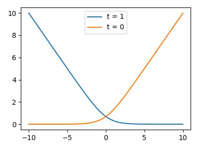
More loss if the prediction is "more" confident about "wrong" answers and not punishing the correct one even not confident

\[\mathcal L_{CE}(y,t) = -t\log(y) - (1-t)\log(1-y)\]

where \(t\in\{0,1\}\)

Logistic Regression¶

\(z = \vec w^T \vec x+b\)
\(y = \sigma(z) = (1+\exp(-z))^{-1}\)
\(\mathcal L_{CE}(y,t) = -t\log(y) - (1-t)\log(1-y)\)

Gradient Descent¶

Initialize the weights to something reasonable and repeated adjust them in the direction of steepest descent

\[\vec w \leftarrow \vec w - \alpha \partial_{\vec w} J\]

\(\alpha \in (0, 1]\) is the learning rate (step size)
When \(J\) converges, \(\partial_{\vec w} J = 0\) at the critical point

Under L² Regularization¶

The gradient descent update to minimize the regularized cost \(\mathcal J + \lambda \mathcal R\) results in weight decay

\[\vec w\leftarrow \vec w - \alpha\partial_{\vec w}(\mathcal J+\lambda \mathcal R) = (1-\alpha\lambda)\vec w - \alpha \partial_{\vec w} \mathcal J\]

Learning rate¶

In gradient descent, the learning rate \(\alpha\) is a hyper parameter. (TUT3)

Training Curves¶

To diagnose optimization problems, plot the training cost as a function of iteration.

However, it's very hard to tell whether an optimizer has converged.

Example: Gradient of logistic loss¶

\[\begin{align*} \frac{\partial\mathcal L_{CE}}{\partial w_j} &= \partial_y \mathcal L_{CE}\cdot \partial_zy \cdot \partial_{wj}z \\ &= (\frac{-t}{y} + \frac{1-t}{1-y})\cdot y(1-y)\cdot x_j\\ &= (y-t)x_j\\ w_j &\rightarrow w_j - \frac{\alpha}{N} \sum^N(y^{(i)} - t^{(i)})x_j^{(i)} \end{align*}\]

Multiclass Classification (Softmax Regression)¶

One-hot vector/ one-of-K encoding Target¶

Targets from a discrete set \(\{1,...,K\}\)
For convenience, let \(t\in\mathbb R^K, t_i= \mathbb I(i=k)\) where \(k\) is the classification.

Linear predictions¶

\(D\) input, \(K\) output, hence we need a weight matrix \(W\)

\[\vec{z}_{K\times 1} = W_{K\times D}\vec{x}_{D\times 1} + \vec{b}_{K\times 1}\]

Otherwise \(Z= Wx^*\) where \(x^*\) is \(x\) padded a column of \(1\)'s.

Softmax Function Activation¶

A generalization of the logistic function

\[y_k = softmax(z_1,...,z_K)_k = \frac{e^{z_k}}{\sum_{k'} e^zk'}\]

The input \(z_k\) are the logits

Properties¶

Outputs are positive and sum to \(1, (\sum_k y_k = 1)\) so that can be interpreted as probabilities
If one of \(z_k\) is much larger, than \(softmax(z)_k \approx 1\)

Cross Entropy Loss¶

Use cross-entropy as the loss function, as from logistic regression

\[\mathcal L_{CE}(\vec y, \vec t) = -\sum_{k=1}^K t_k \log y_k = -\vec t^T \log(\vec y)\]

Log is applied element-wise

Gradient descent¶

Updates can be derived for each row of \(W\)

\[\frac{\partial L}{\partial w_k} = \frac{\partial L}{\partial z_k}\frac{\partial z_k}{\partial w_k} = (y_k - t_k)\cdot \vec x\]

\[w_k \leftarrow w_k - \alpha N^{-1} \sum^N (y^{(i)}_k - t^{(i)}_k)\vec x^{(i)}\]

Source code

import matplotlib.pyplot as plt
import numpy as np

z = np.arange(-10, 10, 0.01)
loss = (np.exp(-z) + 1) ** -1
plt.figure(figsize=(4, 3))
plt.plot(z, loss)
plt.title("logistic function")
plt.tight_layout()
plt.savefig("../assets/classification_logistic.jpg")


plt.figure(figsize=(4, 3))
plt.plot(z, -1 * np.log(loss), label="t = 1")
plt.plot(z, -1 * np.log(1 - loss), label="t = 0")
plt.legend()
plt.tight_layout()
plt.savefig("../assets/classification_loss.jpg")