Density Estimation¶

Histograms¶

Given data \(x_1,...,x_n\) and "bins" \(B_k = [u_{k-1}, u_k), k=1,...,m\), then

Note that \(\text{hist}\) is a pdf since \(\text{hist}(x)\geq 0\) and

Histogram depends on number of bins and boundaries of the bins.

Substitution principle estimation¶

Consider the empirical distribution function

However, we cannot derive any \(f\) since this is not differentiable.

Kernel Density estimation¶

Start with a density function \(w(x)\), i.e. a kernel

Given \(w\) and a bandwidth \(h\), define the kernel density estimator

bandwidth controls the amount of smoothing, as \(h\) increases, the estimator \(\hat f_h(x)\) becomes smoother.

Some examples of kernels are

• Gaussian kernel \(w(x) = \sqrt{2\pi}^{-1}\exp(\frac{-x^2}{2})\)
• Epanechinkov kernel \(w(x) = \frac{3}{4\sqrt 5}(1-\frac{x^2}{5}), |x|\leq \sqrt 5\)
• Rectangular \(w(x) = \frac{1}{2\sqrt{3}}, |x| \leq \sqrt 3\)
• Triangular \(w(x) = \frac{1}{\sqrt 6}(1-\frac{|x|}{\sqrt 6}), |x|\leq \sqrt 6\)

Example¶

Draw 500 observations from

N <- 500
components <- sample(1:2,prob=c(.7, .3),size=N,replace=TRUE)
mus <- c(2, -2)

x <- rnorm(n=N,mean=mus[components],sd=1)
par(mfrow=c(2, 2))
.5387 - plot(density(x))
.8 - plot(density(x, bw=.8))
.4 - plot(density(x, bw=.4))
.2 - plot(density(x, bw=.2))

​

Redistribution¶

The empirical distribution function \(\hat F\) puts probability mass \(1/n\) at each of the points \(X_1,...,X_n\), use the kernel with bandwidth \(h\) to redistribute this mass around each \(X_i\), probability density around \(X_i = \frac{1}{nh}w(\frac{x-X_i}{h})\) where

The density estimate is now simply the sum of these densities over all observations

Convolution¶

Look at the distribution of \(Y_h = U+hV\) where \(U\sim \hat F\) and \(V\) has density \(w\) with \(V,U\) independent. If \(h\) is small then \(Y_h \approx U \sim \hat F\).

Unlike \(U, Y_h\) is a continuous r.v. for each \(h>0\):

Choice of bandwidth¶

The choice of \(h\) depends on what we believe the underlying density looks like, if \(f\) is believed to be smooth, then take larger \(h\). If \(f\) is believed to have a number of modes (i.e. local maxima) then we should take smaller \(h\).

Consider the bias-variance decomposition

As \(h\) decreases, the squared bias term also decrease but the variance increases.

Example: The rectangular kernel¶

Take \(w(x) = 1/2\) for \(|x|\leq 1\). Then,

The mean of \(\hat{f_h}(x)\) is

the squared bias is

For the variance,

Thus, we can approximate the variance by

The MSE is approximately

Uncertainty Estimating¶

Let \((X_1,..., X_n)\sim F_\theta\) for some \(\theta \in \Theta \subset R\), want to estimate \(\theta\) using \(X_1,...,X_n\).

Let \(\hat\theta\) be the estimator of the true \(\theta\), but we don't know what \(\theta\) is, so how can we say about the estimation error?

Example¶

Let \(X_1,...,X_n\) indep. \(N(\mu, \sigma^2)\) random variables. Estimate \(\mu = E(X_i)\) by \(\hat\mu = \bar X\) (substitution principle estimator).

We know that \(\hat\mu \sim N(\mu, \sigma^2/n)\). Then

In this example, knowing the distribution of \(\hat\mu\) tells us a lot about the uncertainty of \(\hat\mu\) of an estimator of \(\mu\).
If \(\sigma^2\) is unknown then we can estimate

and replace 1.96 by some \(t\).

Sampling distribution of \(\hat\theta\) is its probability distribution; this will depend on \(\theta\).

Mean square error of \(\hat\theta\) is defined as

Unbiased if \(bias_\theta(\hat \theta) := E_\theta(\hat\theta) - \theta = 0\)

Problem with unbiasedness¶

• In many problems, unbiased estimators do not exist
• In some problems, the estimator lies outside the parameter space with positive probability
• If \(\hat\theta\) is an unbiased estimator of \(\theta\) and \(g\) is a non-linear function then \(E_\theta[g(\hat\theta)] \neq g(\theta)\) unless \(P_\theta(\hat\theta = \theta) = 1\).

When to worry about bias?¶

• If \(\hat\theta\) is systematically larger or smaller than \(\theta\)
• If the squared bias is approximately equal to or greater than the variance

Example: Sample variance¶

\(X_1,...,X_n\) indep. with \(\mu, \sigma^2\), using unbiased estimator of sample variance

However, \(S = \sqrt{S^2}\) is biased, if we assume that \(X_1,...,X_n\) are Normal then we can evaluate the bias explicitly

Then

Consistency¶

The sequence of estimators \(\hat\theta_n\) is consistent for \(\theta\) if for each \(\epsilon > 0\) and \(\theta\in\Theta\),

a.k.a. \(\hat\theta_n \rightarrow^p \theta\)

Note that consistency is an aspirational property:

• if we have enough info. then we can estimate \(\theta\) arbitrarily precisely.
• For a finite \(n\), consistency isn't meaningful

Sample means and functions thereof¶

\(X_1,...,X_n\) indep. with mean \(\mu\) and \(\sigma^2\), then estimate \(\mu\) by \(\hat\mu_n = n^{-1}\sum_{i=1}^n X_i\)
By WLLN, \(\hat\mu_n\) is a consistent estimator of \(\mu\) (i.e. \(\{\hat\mu_u\}\) is consistent).

Likewise, if we want to estimate \(\theta = g(\mu)\) where \(g\) is a continuous function then \(\hat\theta_n = g(\hat\mu_n)\) is a consistent estimator of \(\theta\).

We can also approximate the sampling distributions of \(\hat\mu_n\) and \(\hat\theta_n\) by normal distributions

Example: Regression design¶

Assume for simplicity that \(\epsilon_1,...,\epsilon_n\) are indep. \(N(0,\sigma^2)\)
Least squares estimator of \(\beta_1\):

Thus \(\hat\beta_1 = \hat\beta_1^{(n)}\) will be consistent provided that

Sampling distributions and standard errors¶

Assume \(\hat\theta\) is an estimator of some parameter \(\theta\), then \(se(\hat\theta)\) is defined to be the standard deviation of the sampling deviation of the sampling distribution of \(\hat\theta\).
This is rarely known exactly but can usually be approximated somehow.

If \(\hat\mu = \bar X\) where \(\bar X\) is based on \(n\) indep. observations with variance \(\sigma^2\) then \(se(\hat\mu) = \sigma/\sqrt n\).

If the sampling distribution is approximately normal then we can approximate the standard error by the standard deviation of the approximating normal distribution.

Example¶

\(\hat\mu = \bar X, se(\hat\mu) = \sigma/\sqrt n\). estimated standard error is

Example: the Delta Method estimator¶

\(X_1,...,X_n\) indep. with some unknown cdf \(F\), suppose \(\hat\theta = g(\bar X)\).
If \(g\) is differentiable then we can approximate the sampling distribution of \(\hat\theta\) by a normal distribution using Delta Method:

where \(\sigma^2 = var(X_i)\) This suggests that we can estimate \(se(\hat\theta)\) using the Delta Method estimator

where \(S^2\) is the sample variance of \(X_1,...,X_n\).
We are using the substitution principle here to estimate the unknown \(\mu\) and \(\sigma^2\)

Recall that the Delta Method follows from the Taylor series approximation

Thus

We "estimate" \(\phi(X_i)\) by a pseudo-value

Note that

The Delta Method estimator can now be written as

Example: Trimmed mean¶

\(X_1,...,X_n\) indep. continuous r.v. with density \(f(x-\theta)\) where \(f(x) = f(-x)\) and \(\theta\) is unknown. if suspecting that \(f\) is heavy-tailed, then we want to eliminate the effects of extreme observations.

To minimize the effect of extreme observations, we estimate \(\theta\) by a trimmed mean:

In general, the trimmed mean is a substitution principle estimator of

where \(a = r/n\).

Then, the sampling distribution of trimmed mean is approximately normal

where

Approximating estimators by sample means¶

Suppose that \(\hat\theta\) is some complicated estimator like a trimmed mean.

How to compute \(\hat{se}(\hat\theta)\), suppose that we can approximate \(\hat\theta\) by an average \(\hat\theta \approx n^{-1}\sum^n \phi(X_i)\)

This suggests using

where \(\bar\phi = \frac1n \sum^n \phi(X_i)\approx \hat\theta\)

Leave-one-out estimators¶

Suppose that \(\hat\theta = \hat\theta(X_1,...,X_n)\), then define \(\hat\theta_{-i} = \hat\theta(X_1,...,X_{i-1}, X_{i+1},...,X_n)\)
if \(\hat\theta = \bar X\) then \(\hat \theta_{-i} = \frac1{n-1}\sum_{j\neq i}X_j\)

Example: Theil Index¶

Define \(\theta(F) = E_F[\frac{X_i}{\mu(F)}\ln (\frac{X_i}{\mu(F)})]\) where \(P(X_i > 0) = 1\) and \(\mu(F) = E_F(X_i)\).

We estimate \(\theta(F)\) by

The leave-one-out estimators are

where \(\bar X_{-i} = \frac1{n-1}\sum_{j\neq i}X_j\)

From leave-one-out to pseudo-values¶

Suppose that we can approximate \(\hat\theta\) by a sample mean

for some (unknown) function \(\phi\).

Then for the leave-one-out estimators, we have

This suggests that we can recover \(\phi(X_i)\) (approximately) by the pseudo-value

The pseudo-values can be used to estimate the s.e. of \(\hat\theta\).

Jackknife s.e. estimator¶

Given the pseudo-values \(\Phi_1,...,\Phi_n\), define the jackknife estimator of \(se(\hat\theta)\)

where \(\hat\theta_\cdot = \frac1n \sum^n \hat\theta_{-i}\)
For many estimators, we have

We can use the jacknife to remove the \(1/n\) bias term.

Define the bias-corrected \(\hat\theta\):

For \(\hat\theta_{bc}\), then

x <- rgamma(100,2)
y <- x/mean(x)
theil <- mean(y*log(y))
sprintf("theil index %f", theil)
# Compute pseudo-values
pseud <- NULL
for (i in 1:100) {
    xi <- x[-i]
    yi <- xi/mean(xi)
    loo <- mean(yi*log(yi))
    pseud <- c(pseud,100*theil - 99*loo)
}
sprintf("mean of pseudo %f", mean(pseud)) # mean of pseudo-values - bias-corrected estimate
sprintf("jackknife s.e. estimate %f", sqrt(var(pseud)/100))

theil index 0.188827
mean of pseudo 0.190167
jackknife s.e. estimate 0.022019

Delta Method vs. Jackknife¶

Sample 100 observations from a Gamma distribution with \(\alpha = 2\) and \(\lambda = 1\).
Estimate \(\theta = \ln(\mu) = g(\mu); g'(\mu) = 1/\mu\). For our sample \(\bar x = 1.891\) and \(s^2 = 1.911\), \(\hat \theta = \ln(\bar x) = 0.637\)

Thus the Delta Method s.e. estimate is

Computing the jackknife estimate is somewhat more computationally intensive.

x <- rgamma(100,2)
thetaloo <- NULL
for (i in 1:100) {
    xi <- x[-i]
    thetaloo <- c(thetaloo,log(mean(xi)))
}
jackse <- sqrt(99*sum((thetaloo-mean(thetaloo))^2)/100)
sprintf("jackkniefe s.e. %f", jackse)

jackkniefe s.e. 0.070312

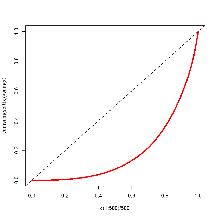
Example: The Lorenz curve¶

Suppose that \(F\) is the cdf of a positive r.v. with finite mean \(\mu(F)\), let \(F\) describes the income distribution within some population.

For each such \(F\), we can define its Lorenz curve:

a.k.a. the fraction of total income held by poorest \(\tau\).

\(\mathcal L_F(\tau) \leq \tau\) with \(\mathcal L_F(0) = 0\) and \(\mathcal L_F(1)=1\).
The difference between \(\tau\) and \(\mathcal L_F(\tau)\) can be used to measure income inequality.

Example: The Gini index¶

One measure of income inequality is the Gini index defined by

\(Gini(F)\in [0,1]\Rightarrow 0\) perfect equality, \(1\) perfect inequality.

We estimate the quantiles \(F^{-1}(\tau)\) by order statistics. Given indep. observations \(X_1,...,X_n\) from \(F\), we have

gini <- function(x) {
    # compute point estimate
    n <- length(x)
    x <- sort(x)
    wt <- (2*c(1:n)-1)/n - 1
    g <- sum(wt*x)/sum(x)
    # compute leave-one-out estimates
    wt1 <- (2*c(1:(n-1))-1)/(n-1) - 1
    gi <- NULL
    for (i in 1:n) {
        x1 <- x[-i] # data with x[i] deleted
        gi <- c(gi,sum(wt1*x1)/sum(x1))
    }
    # compute jackknife std error estimate
    gbar <- mean(gi)
    se <- sqrt((n-1)*sum((gi-gbar)^2)/n)
    r <- list(gini=g,se=se)
}

# generate 500 observations from a Gamma( a = 1/2 )
x <- rgamma(500,1/2) # Sample from a Gamma with alpha=1/2
r <- gini(x)
sprintf("gini %f", r$gini)
sprintf("s.e. %f", r$se)

gini 0.626679
s.e. 0.012652

plot(c(1:500)/500,cumsum(sort(x))/sum(x),type="l",lwd=4,col="red")
abline(0,1,lty=2,lwd=2)

​