Scale Invariant Feature Transform

import cv2
import numpy as np
from matplotlib import pyplot as plt
import seaborn as sns

def imshow(img, ax=None, title="", bgr=True):
    # since plt and cv2 have different RGB sorting
    if bgr:
        img = cv2.cvtColor(img,cv2.COLOR_BGR2RGB)
    if ax == None:
        plt.imshow(img.astype(np.uint8))
        plt.axis("off")
        plt.title(title)
    else:
        ax.imshow(img.astype(np.uint8), cmap="gray")
        ax.set_axis_off()
        ax.set_title(title)

plt.rcParams["figure.figsize"] = (12,6)

Distinctive Image Features from Scale-Invariant Keypoints [David G. Lowe, 2004]

LoG and DoG

Laplacian of Gaussian

Let \(G\) be the Gaussian function, \(G = (2\pi\sigma^2)^{-1} \exp(-\frac{x^2+y^2}{2\sigma^2})\)

\[\begin{align*} \frac{\partial G}{\partial x} & (2\pi\sigma^2)^{-1} \exp(-\frac{x^2+y^2}{2\sigma^2}) \frac{-x}{\sigma^2}\\ \frac{\partial^2G}{\partial x^2} &= (2\pi\sigma^2)^{-1} \big[\exp(-\frac{x^2+y^2}{2\sigma^2})\frac{-x^2}{\sigma^4} + \exp(-\frac{x^2+y^2}{2\sigma^2})\frac{-1}{\sigma^2}\big] \\ &= (2\pi\sigma^2)^{-1} \frac{x^2 - \sigma^2}{\sigma^4} \exp(-\frac{x^2+y^2}{2\sigma^2})\\ \nabla^2 G &= \frac{\partial^2G}{\partial x^2} + \frac{\partial^2G}{\partial y^2} \\ &= (2\pi\sigma^2)^{-1} \frac{x^2 - 2\sigma^2 + y^2}{\sigma^4} \exp(-\frac{x^2+y^2}{2\sigma^2}) \end{align*}\]

Difference of Gaussian

\[\begin{align*} \frac{\partial G}{\partial \sigma} &= \frac{-1}{\pi\sigma^3}\exp(-\frac{x^2+y^2}{2\sigma^2}) + \frac{1}{2\pi\sigma^2}\exp(-\frac{x^2+y^2}{2\sigma^2})\frac{x^2+y^2}{\sigma^3} \\ &= (2\pi\sigma^2)^{-1}\exp(-\frac{x^2+y^2}{2\sigma^2})(\frac{x^2+y^2}{\sigma^3}-\frac{2\sigma^2}{\sigma^3})\\ &= (2\pi\sigma^2)^{-1}\exp(-\frac{x^2+y^2}{2\sigma^2})(\frac{x^2+y^2}{\sigma^4}-\frac{2\sigma^2}{\sigma^4})\sigma\\ &= \sigma\nabla^2G \end{align*}\]

By the limit definition of derivative,

\[\frac{\partial G}{\partial \sigma} = \lim_{h\rightarrow 0} \frac{G(x,y, \sigma+h) - G(x, y,\sigma)}{h}\approx lim_{k\rightarrow 1} \frac{G(x,y, k\sigma) - G(x, y,\sigma)}{(k-1)\sigma}\]

So that

\[DoG := G(x,y, k\sigma) - G(x, y,\sigma) \approx (k-1)\sigma\sigma \nabla^2G = (k-1)\sigma^2 \nabla^2G\]

Scale-space extrema (Octave)

To identify locations and scales that can be repeatably assigned under differing views of the same object.

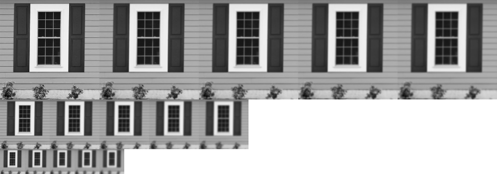
Constructing octave

Generate \(m\) octaves (or image pyramids), each with \(n\) different blurring scale (\(k^1\sigma, ..., k^n\sigma\)). Generally, we choose \(k = 2^{1/s}, s\in\mathbb Z\), and each octave contains \(s+3\) scales, i.e. \(2^{1/s}, 2^{2/s},...2^{1+3/s}\). Then, for the next level of the octave, down-sample from the one with \(2\sigma\), then keep do the next.

Example If \(s = 2\), i.e. \(k = \sqrt{2}\)

	scale1	scale2	scale3	scale4	scale5
octave1	\(\sqrt{2}\)	\(2\)	\(2\sqrt{2}\)	\(4\)	\(4\sqrt{2}\)
octave2	\(2\sqrt{2}\)	\(4\)	\(4\sqrt{2}\)	\(8\)	\(8\sqrt{2}\)
octave3	\(4\sqrt{2}\)	\(8\)	\(8\sqrt{2}\)	\(16\)	\(16\sqrt{2}\)
octave4	\(8\sqrt{2}\)	\(16\)	\(16\sqrt{2}\)	\(32\)	\(32\sqrt{2}\)

Note that \(G(0, \sigma_1)* G(0, \sigma_2) = G(0, \sqrt{\sigma_{1}^2 + \sigma_{2}^2})\) so that within one octave, we continously convolve the image with scale \(k\). Also, downsampling by \(s\) will divide the current scale by \(s\).

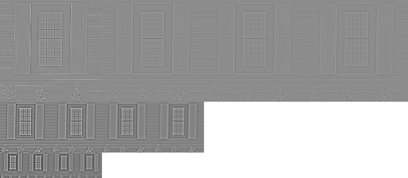
Taking DoG

Then, for each octave, take DoG by taking the difference between adjacent scales. Note that \(k\) is unchanged for each DoG. Then, decide the matching frequency and record the matching.

Find Local Extrema

Find the local extrema by searching each scale in each octave, except the first and last scale, i.e. \(1,...,s+1\). "Localization" means the 8 pixels around it, 9 pixels above it, and 9 pixels below it.

Key Points Localization (orientation invariant)

For each chosen local extrema point, apply Harris corner detector with appropriate window size to remove all the edges and flats.