Linear Filters

Images

Denote a image (matrix of integer values) as \(I\)
For gray-scale images, \(I_{m\times n}\); where \(I(i,j)\) is called intensity
For color images, \(I_{m\times n\times \{1,2,3\}}\), 3 for RGB values

Alternatively, think of a grayscale image as a mapping \(I:\mathbb N^2 \rightarrow \{0,1,...,255\}\), i.e. position \((i,j)\rightarrow\) gray-scale, where 0 is black, 255 is white

Example For image \(I(i,j)\); \(I(i,j)+50\) lighten the image, \(I(i,-j)\) rotate the image horizontally

Image filters

Modify the pixels in an image based on some function of a local neighborhood of each pixel

Can be used to enhance (denoise), detect patterns (matching), extract information (texture, edges)

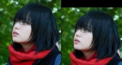
Boundary Effects

Consider the boundary of the image, there are three modes: full, same, valid

Correlation

Given a image \(I\), the filtered image is

\[G(i,j) = \sum_{u=-k}^k \sum_{v=-k}^k F(u,v)\cdot I(i+u, j + v)\]

The entries of the weight kernel of mask \(F(u,v)\) are often called the filter coefficients
Denote this correlation operator \(F\otimes I\)

OpenCV cv2.filter2d

We can also write correlation in a more compact form using vectors, i.e.

Let \(\mathbf f = F\) be the kernel matrix, \(\mathbf t_{ij} = T_{i,j}(I_{\{i-k, i+k\} \times \{j-k, j+k\}})\) be the matrix of the image centered at \((i,j)\) and of size \(2k + 1\), then \(G(i,j)=\mathbf f\cdot \mathbf t_{ij}\)

And the full image

\[\mathbf G_{m\times n} = \begin{bmatrix} G(0,0) &G(0, 1)&\cdots &G(0, n) \\ G(1,0) &G(1, 1)&\cdots &G(1, n) \\ \vdots &\vdots&\ddots &\vdots \\ G(m,0) &G(m, 1)&\cdots &G(m, n) \\ \end{bmatrix}\]

Example of Filter kernels

Unchanged

\(\begin{bmatrix} 0 &0 &0 \\ 0 &1 &0 \\ 0 &0 &0 \end{bmatrix}\)

shifting to the left by 1px

\(\begin{bmatrix} 0 &0 &0 \\ 0 &0 &1 \\ 0 &0 &0 \end{bmatrix}\)

Sharpening

\[M1 = \begin{bmatrix} 0 &0 &0 \\ 0 &2 &0 \\ 0 &0 &0 \end{bmatrix} - \frac{1}{9} \begin{bmatrix} 1 &1 &1 \\ 1 &1 &1 \\ 1 &1 &1 \end{bmatrix}\]

To enhance the effect, using a larger center value

\[M2 = \begin{bmatrix} 0 &0 &0 \\ 0 &5 &0 \\ 0 &0 &0 \end{bmatrix} - \frac{4}{9} \begin{bmatrix} 1 &1 &1 \\ 1 &1 &1 \\ 1 &1 &1 \end{bmatrix}\]

If we enlarge the matrix to 5

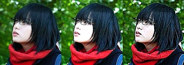
\[M3 = \vec 0_{5\times 5} + [5]_{center} - \frac{4}{25} J_{5\times 5}\]

Smoothing

Smoothing 1: Moving Averaging filter

Simplest thing is to replace each pixel by the average of its neighbors, i.e. \(F\) will be a \((2k+1)^{-2} J_{(2k+1)\times (2k+1)}\) matrix

Assumption neighboring pixels are similar, and noise is independent of pixels.

For example, the following uses \(\frac{1}{9}J_{3\times 3}\) and \(\frac{1}{25}J_{5\times 5}\), note that the matrix should add up to one, hence the image is normalized.

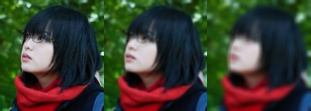
Smoothing 2: Gaussian Filter

When we want nearest neighboring pixels to have the most influence on the output, which can removes high-frequency components from the image (low-pass filter).

For example,

\[F = \frac{1}{16} \begin{bmatrix} 1 &2 &1 \\ 2 &4 &2 \\ 1 &2 &1 \end{bmatrix}\]

The Gaussian kernel is an approximation of a 2d Gaussian function

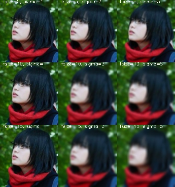
\[h_{\sigma}(u,v)=\frac{1}{2\pi \sigma^2}\exp(-\frac{u^2 + v^2}{\sigma^2})\]

A more general form of the Gaussian kernel is obtained by the multi-variante Gaussian distribution \(\mathcal N(\mu, \Sigma)\), where

\[P(\vec x) = \frac{1}{(2\pi)^{d/2} |\Sigma|^{1/2}} \exp(-\frac{(\vec x - \mu)^T \Sigma^{-1}(\vec x - \mu)}{2})\]

Properties of Smoothing

All values are positive
The kernel sums up to 1 to prevent re-scaling of the image
Remove high-frequency components (edges); low-pass filter

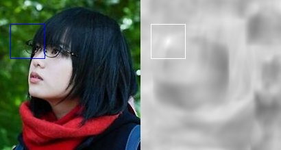
Filtering image to find image crop (Normalized cross-correlation)

Let \(\mathbf f\) be a image crop, \(\mathbf t\) be the original image, then

\[G(i,j) = \frac{\mathbf f^T \mathbf t_{ij}}{\|\mathbf f^T \|\|\mathbf t_{ij}\|}\]

is the "normalized score" \((0\sim 1)\), where \(1\) indicates the matching

Consider the following image crop

Convolution

A convolution \(F*I\) is equivalent to flip \(F\) along the diagonal and apply correlation. i.e.

\[G(i,j) = \sum_{u=-k}^k\sum_{v={-k}}^k F(u,v)\cdot I(i-u, j-v)\]

Obviously, for a symmetric filter matrix, convolution and correlation will do the same

Convolution is the natural linear feature, and it is

commutative \(f*g = g*f\),
associative \(f*(g*h) = (f*g)*h\),
distributive \(f*(g+h)=f*g + f*h\)
associative with scalar \(\lambda (f*g)=(\lambda f)*g\)
The Fourier transform of two convolved images is the product of their individual Fourier transforms \(\mathcal F(f*g) =\mathcal F(f)\cdot \mathcal F(g)\)

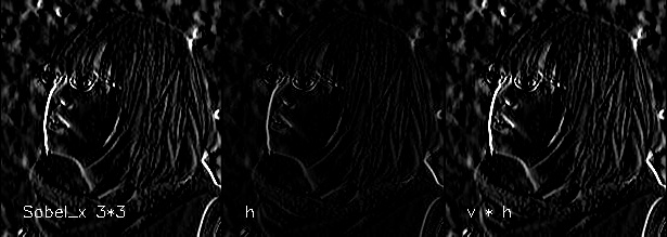
Separable Filters

A convolution filter is separable if it can be written as the outer product of two 1D filters. i.e. \(F = vh^T\), then \(F*I = v*(h*I)\) by associative property.

Example

\[ k^{-2} J = k^{-1}[1 \:1 \:... \:1]^T k^{-1}[1 \:1 \:... \:1]\]

\[ \frac{1}{16} \begin{bmatrix} 1 &2 &1 \\ 2 &4 &2 \\ 1 &2 &1 \end{bmatrix} = \frac{1}{4} \begin{bmatrix} 1\\ 2\\ 1 \end{bmatrix} \frac{1}{4} \begin{bmatrix} 1&2&1 \end{bmatrix}\]

\[ \begin{bmatrix} -1 &0 &1 \\ -2 &0 &2 \\ -1 &0 &1 \end{bmatrix} = \begin{bmatrix} 1\\ 2\\ 1 \end{bmatrix} \begin{bmatrix} -1&0&1 \end{bmatrix}\]

How to tell is separable

Quickcheck it has rank 1 (otherwise it cannot be written as 2 1D array)

Singular value decomposition (SVD) decompose by \(F = \mathbf U \Sigma \mathbf V^T = \sum_i \sigma_i u_i v_i^T\) with \(\Sigma = diag(\sigma_i)\) if only one singular value \(\sigma_i\) is non-zero, then it is separable and \(\sqrt{\sigma_1}\mathbf u, \sqrt{\sigma_1} \mathbf v_1^T\) are the 1D filters

Source code