Multi Comparisons and One Way ANOVA
Multiple Comparisons
- post hoc procedure: further comparisons after significant result from overall One-way ANOVA
- If the result for One-way ANOVA is good enough, i.e.some pairs are evidently true, we may omit some pairs to remove the number of tests
- Max of \(G \choose 2\) pairwise comparisons
- Major issue: increased chance of making at least one Type I error when carrying out many tests, \(E(\#errors)=\#tests \times \alpha\)
- Two common solutions: based on controlling family Type I error rate, choose
- Bonferroni
- Tukey's
Example \(P(\text{committing at least 1 Type I error})\) ?
- For n independent tests: \(P = 1-(1-\alpha)^n\)
Bonferroni's Method
- Based on Bonferroni's inequality \(P(A\cup B) \leq P(A)+P(B)\), hence \(P(\cup A_i)\leq \sum P(A_i), A_i:=\) the event that \(i\)th test results in a Type I error.
- Method: conduct each of \(k=G \choose 2\) pairwise tests at level \(\alpha / k\)
- CI: \(|\bar{y}_i - \bar{y}_j|\pm t_{\alpha/2k} S_p \sqrt{n_i^{-1} + n_j^{-1}}\)
- Conservative: overall Type I error rate is usually much less than \(\alpha\) if tests are not mutually independent.
- Type II error inflation.
Tukey's Approach
- Usually less conservative than Bonferroni, particularly if group sample size are similar. Controls the overall Type I error rate of \(\alpha\), simultaneous CI converage rate is \(1-\alpha\).
Studentized Range distribution
- \(\mathcal{X}= \{X_1,...,X_n\}, X_i\in N(\mu,\sigma^2)\). Determine the distribution of the max and min of \(\mathcal{X}\).
- \(X_{(n)}:=\max{\mathcal{X}}, X_{(1)};=\min{\mathcal{X}}\), Range \(:= X_{(n)}-X{(1)}\)
- Based on \(n\) observations from \(X\), the Studentized range statistic is \(Q_{stat} = Range / s, s=\) sample std.
-
Based on \(G\) group means, with \(n\) observations per group:
\[\bar{Q}_g = \frac{\sqrt{n}(\bar{y}_{(g)} - \bar{y}_{(1)})}{s_v}\]
\(s_v\) estimator of the pooled std. \(v=N-G=G(n-1)\) d.f.
- If there are \(G\) groups, then there is a max of \(k\) pairwise differences
- Controlling overall simultaneous Type I error rate v.s. Individual Type I error rate
- Find a pairwise significant difference
- Compare method-wise significant difference, \(c(\alpha)\) with \(|\bar{y}_i - \bar{y}_j|\) OR
- determine whether CI contains 0 OR
- Compare \(p\) with \(\alpha\)
- \(s=\sqrt{MSE}\) with d.f. \(=v=d.f.Error\)
Tukey's Honestly Significant Difference (HSD)
- let \(q(G,v,\alpha)/t^*:=\) the critical value from the Studentized Range distribution.
- Family rate \(=\alpha\)
- Tukey's HSD \(=q(G,v,\alpha) \frac{s}{\sqrt{n}}\)
Case Study
Bonferroni
- \(H_0:\mu_i - \mu_j = 0, H_a: \mu_i\neq \mu_j\)
- \(t = \frac{\bar{x}_i - \bar{x}_j}{S_p \sqrt{n_i^{-1} + n_j^{-1}}}\)
- \(p = 2P(T_{\alpha/2k}> |t|)\)
    Pairwise comparisons using t tests with pooled SD

data:  percent and judge

  Spock's A       B       C       D       E
A 0.00022 -       -       -       -       -
B 0.00013 1.00000 -       -       -       -
C 0.00150 1.00000 1.00000 -       -       -
D 0.57777 1.00000 1.00000 1.00000 -       -
E 0.03408 1.00000 1.00000 1.00000 1.00000 -
F 0.01254 1.00000 1.00000 1.00000 1.00000 1.00000

P value adjustment method: bonferroni
| 0.357 % | 99.643 % | |
|---|---|---|
| (Intercept) | 8.078085 | 21.16636 |
| judgeA | 8.547341 | 30.44821 |
| judgeB | 8.647254 | 29.34163 |
| judgeC | 5.222969 | 23.73259 |
| judgeD | -2.969585 | 27.72514 |
| judgeE | 1.997255 | 22.69163 |
| judgeF | 2.922970 | 21.43259 |
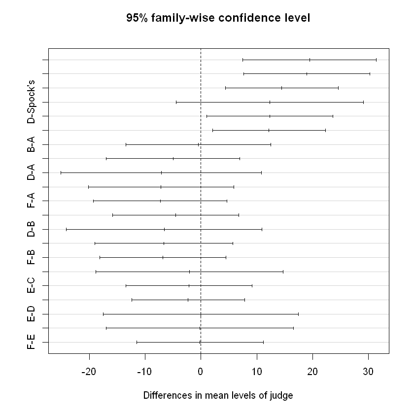
  Tukey multiple comparisons of means
    95% family-wise confidence level

Fit: aov(formula = percent ~ judge)

$judge
                 diff        lwr       upr     p adj
A-Spock's 19.49777727   7.514685 31.480870 0.0001992
B-Spock's 18.99444405   7.671486 30.317402 0.0001224
C-Spock's 14.47777732   4.350216 24.605339 0.0012936
D-Spock's 12.37777758  -4.416883 29.172438 0.2744263
E-Spock's 12.34444443   1.021486 23.667402 0.0248789
F-Spock's 12.17777766   2.050216 22.305339 0.0098340
B-A       -0.50333322 -13.512422 12.505755 0.9999997
C-A       -5.01999995 -17.003092  6.963092 0.8470098
D-A       -7.11999969 -25.094638 10.854639 0.8777485
E-A       -7.15333284 -20.162421  5.855755 0.6146239
F-A       -7.31999961 -19.303092  4.663093 0.4936380
C-B       -4.51666673 -15.839625  6.806291 0.8742030
D-B       -6.61666648 -24.158118 10.924785 0.9003280
E-B       -6.64999962 -19.053679  5.753679 0.6418003
F-B       -6.81666639 -18.139624  4.506292 0.5109582
D-C       -2.09999975 -18.894661 14.694661 0.9996956
E-C       -2.13333289 -13.456291  9.189625 0.9968973
F-C       -2.29999966 -12.427561  7.827562 0.9914731
E-D       -0.03333314 -17.574784 17.508118 1.0000000
F-D       -0.19999992 -16.994661 16.594661 1.0000000
F-E       -0.16666677 -11.489625 11.156291 1.0000000
Linear Regression Model
- \(Y_{N\times 1}=X_{N\times(p+1)}\beta_{(p+1)\times 1} + \epsilon_{N\times 1}\), response \(Y\) continuous, explanatory \(X\) categorical and/or continuous
- \(Y\) is linear in the \(\beta\)'s i.e. no predictor is a linear function or combination of other predictors
- \(\hat{\beta}=(X'X)^{-1}X'Y\) Least square Estimate, need\(rank(X'X)=rank(X)\Rightarrow\) columns of \(X\) must be linear independent
- Null hypothesis \(H_0: \beta = \vec{0}\). Assumptions
- Appropriate Linear Model
- Uncorrelated Errors
- \(\vec{\epsilon}\sim N(\vec{0},\sigma^2I)\).
-
Sum of Squares Decomposition
\[\begin{align*}SST&=SSE+SSR\\ \sum_i^N(Y_i-\bar{Y})^2 &= \sum_i^N (Y_i-\hat{Y}_i)^2 + \sum_i^N(\hat{Y}_i - \bar{Y})^2 \end{align*}\]
One-Way ANOVA
- Need one factor (categorical variable) with at least 2 levels \((G\geq 2)\)
-
Aim: Compare \(G\) group means
\[H_0:\mu_1=\mu_2=...=\mu_G, H_a:\exists i\neq j. \mu_i\neq \mu_j\] -
Predictors are indicator variables that classify the observations one way (into \(G\) groups)
- special case of a general linear model
- equivalent to GLM with one-way classification (one factor)
- GLM uses \(G-1\) dummy variables
- ANOVA: compare means by analyzing variability
One Way Expectations and Estimates
Then, the null hypothesis is \(H_0: \beta_i=\mu_i-\mu_0 = 0\Rightarrow\) the equal mean of \(i\)th group and the compared group
In this case, for \(SST\), \(N=\sum_1^G n_i,\hat{Y}_i=\) mean of observations for group \(g\) from which the \(i\)th observation belongs, \(\bar{Y}=\frac{\sum_{g=1}^{G}\sum_{j=1}^{n_g} y_{gj}}{N}\) is the grand mean
judge
Spock's       A       B       C       D       E       F
      9       5       6       9       2       6       9
Spock's     14.6222224235535
A           34.1199996948242
B           33.6166664759318
C           29.0999997456868
D           27
E           26.9666668574015
F           26.800000084771
Compare 6 judges (exclude Spock)
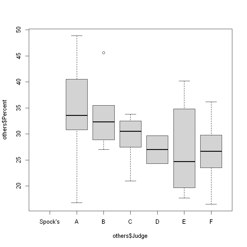
             Df Sum Sq Mean Sq F value Pr(>F)
others$Judge  5  326.5   65.29   1.218  0.324
Residuals    31 1661.3   53.59
Rule of thumb
Not a formal way, not a quick check whether equal variance
Spock's     <NA>
A           11.9418181005452
B           6.58222301297842
C           4.59292918339244
D           3.81837769736668
E           9.01014223675898
F           5.96887758208529
11.9418181005452
3.81837769736668
TRUE
    Bartlett test of homogeneity of variances

data:  others$Percent and others$Judge
Bartlett's K-squared = 6.3125, df = 5, p-value = 0.277
The small p-value may due to the uneven and small group sizes
Compare all 7 judges
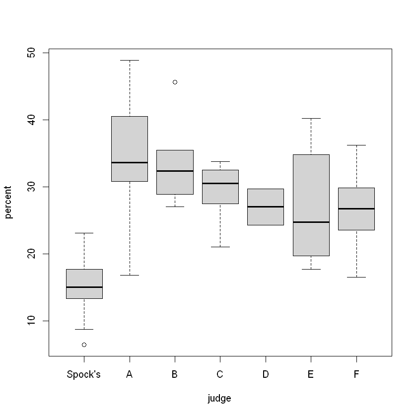
            Df Sum Sq Mean Sq F value  Pr(>F)
judge        6   1927   321.2   6.718 6.1e-05 ***
Residuals   39   1864    47.8
---
Signif. codes:  0 '***' 0.001 '**' 0.01 '*' 0.05 '.' 0.1 ' ' 1
Call:
lm(formula = percent ~ judge)

Residuals:
    Min      1Q  Median      3Q     Max
-17.320  -4.367  -0.250   3.319  14.780

Coefficients:
            Estimate Std. Error t value Pr(>|t|)
(Intercept)   14.622      2.305   6.344 1.72e-07 ***
judgeA        19.498      3.857   5.056 1.05e-05 ***
judgeB        18.994      3.644   5.212 6.39e-06 ***
judgeC        14.478      3.259   4.442 7.15e-05 ***
judgeD        12.378      5.405   2.290 0.027513 *
judgeE        12.344      3.644   3.388 0.001623 **
judgeF        12.178      3.259   3.736 0.000597 ***
---
Signif. codes:  0 '***' 0.001 '**' 0.01 '*' 0.05 '.' 0.1 ' ' 1

Residual standard error: 6.914 on 39 degrees of freedom
Multiple R-squared:  0.5083,    Adjusted R-squared:  0.4326
F-statistic: 6.718 on 6 and 39 DF,  p-value: 6.096e-05
Spock's     5.03879411343757
A           11.9418181005452
B           6.58222301297842
C           4.59292918339244
D           3.81837769736668
E           9.01014223675898
F           5.96887758208529
TRUE
    Bartlett test of homogeneity of variances

data:  percent by judge
Bartlett's K-squared = 7.7582, df = 6, p-value = 0.2564
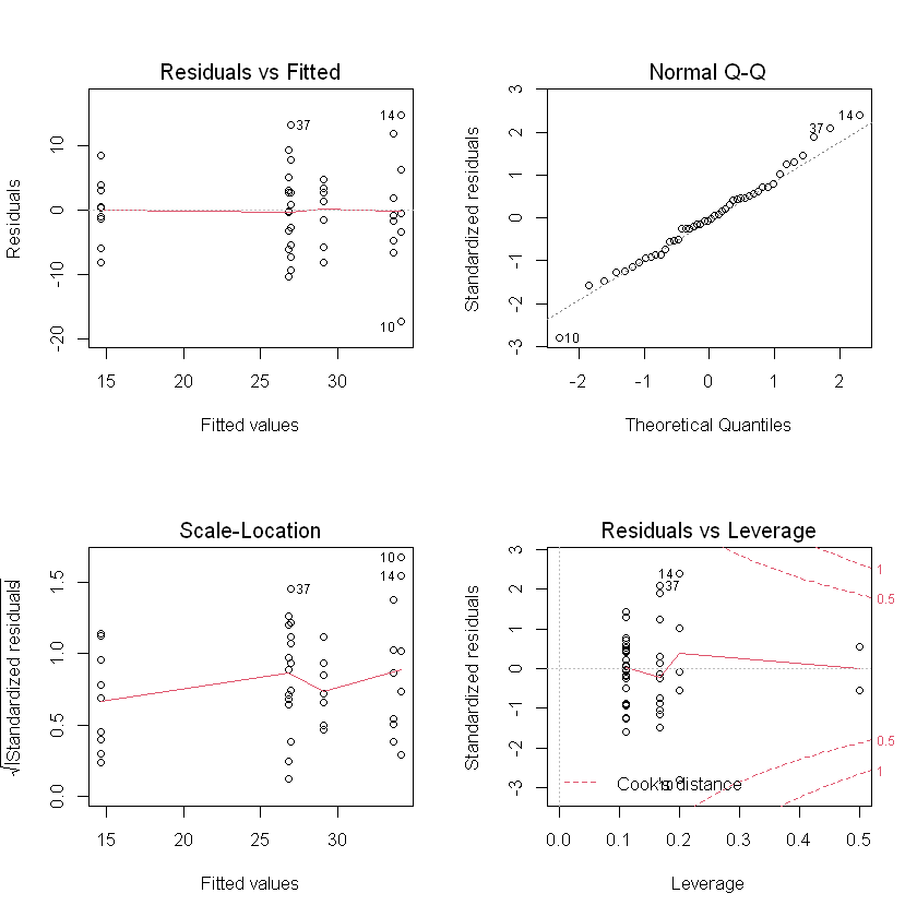
- Residual vs Fitted: No obvious pattern, assume equal variance (also by rule of thumb and Bartlett)
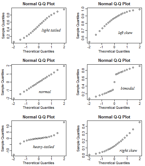
- Normal Q-Q: overall OK
- Outliers: see Residual vs leverage, not influential point.