Spacings
Given the order statistics \(X_{(1)}\leq ... \leq X_{(n)}\), define \((n-1)\) spacings (first order spacings) by
Intuitively, the spacings should carry some information about the pdf \(f\).
Note that if \(\tau \approx \frac{k+1}{n}\approx \frac{k}{n}\) then \(X_{(k+1)}\) and \(X_{(k)}\) estimate \(F^{-1}(\tau)\).
If \(f(F^{-1}(\tau))\) is large then \(D_k\) is small, conversely, \(f(F^{-1}(\tau))\) is small then \(D_k\) is large.
Exponential Spacings
\(X_1,...,X_n\sim Exp(\lambda)\) iid.
Given the order statistics \(X_{(1)}\leq ...\leq X_{(n)}\) define
Proposition 1
\(Y_1,...,Y_n\) are iid \(\sim Exp(\lambda)\)
proof. Note that the join pdf of \((X_{(1)}, ..., X_{(n)})\) if
Also, note that
Therefore,
Note that \(|J|\) is the absolute determinant of the matrix
which is \(\frac{1}{n!}\)
Proposition 2
If \(\frac{k_n}n\rightarrow\tau\in (0,1)\) and \(f(F^{-1}(\tau)) > 0\), then
proof. Note that
where \(E_i \sim Exp(1)\)
so that
Example: density estimation using spacings
Consider \(D_1,...,D_{n-1}\) are iid. exponential with \(E(nD_k) = \exp(g(V_k))\) where \(V_k = \frac{X_{(k+1)} + X_{(k)}}{2}\), then \(V_k\approx F^{-1}(\tau), \tau\approx \frac kn\approx \frac{k+1}n\) and the density is \(f(x)=\exp(-g(x))\)
Using B-spline functions, we can estimate the function \(g(x)\)
where \(\beta_i\)'s are unknown parameters and \(\psi_j\)'s are B-spline functions.
# create the splines functions
den.splines <- function(x,p=5) {
    library(splines)
    n <- length(x)
    x <- sort(x)
    x1 <- c(NA,x)
    x2 <- c(x,NA)
    sp <- (x2-x1)[2:n]
    mid <- 0.5*(x1+x2)[2:n]
    y <- n*sp
    xx <- bs(mid,df=p)
    r <- glm(y~xx,family=quasi(link="log",variance="mu^2"))
    density <- exp(-r$linear.predictors)
    r <- list(x=mid,density=density)
    r
}
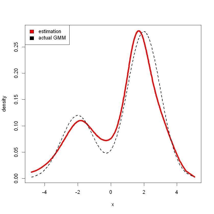
Consider sampling from GMM model
# randomly sample 500 points from given GMM
x <- ifelse(runif(500) < .7, rnorm(500, 2, 1), rnorm(500, -2, 1))
# estimate density using p = 8
r <- den.splines(x,p=8)
# estimation
plot(r$x,r$density,type="l",xlab="x",ylab="density",lwd=4,col="red")
# actual
lines(r$x,0.3*dnorm(r$x,-2,1)+0.7*dnorm(r$x,2,1),lwd=2,lty=2)
legend("topleft", c("estimation", "actual GMM"), fill=c("red", "black"))
Hazard Functions
For \(X\) is a positive continuous rv, its hazard function is
The motivation behind is to consider \(X\) as the survival time, consider
Therefore, this represents instantaneous death rate given survival to time \(x\).
Also, note that
Therefore,
In this case, we require \(\int_0^\infty h(x)dx = \infty\) so that to have a "proper" probability distribution.
The shape of the hazard function gives info not immediately apparent in \(f\) or \(F\). \(h(x)\) increasing indicates new better than used, decreasing indicates used better than new