Order Statistics

Let \(X_1,...,X_n\) indep. with unknown \(F\)

order \(X_1,...,X_n\) in increasing order \(X_{(1)}\leq ... \leq X_{(n)}\). Due to the independence assumption, the order statistics carry the same info about \(F\) as the unordered.

Also, the order statistics can be used to estimate the quantiles \(F^{-1}(\tau)\), such as median

\[M = \begin{cases} \frac{1}{2}(X_\frac n2 + X_{\frac n2+1}) &\text{even}\\ \frac 1 2 X_{\frac{n+1}2} &\text{odd} \end{cases}\approx F^{-1}(1/2)\]

Similarly, \(F^{-1}(\tau)\approx X_{k}, k \approx \tau n\)

Sample Extremums

with the independence assumption,

Sample Minimum

\[\begin{align*} P(X_{(1)}\leq x) &= 1 - P(X_{1}>x)\\ &= 1 - P(X_1>x, X_2>x,..., X_n>x)\\ &= 1 - \prod_{i=1}^n P(X_i>x) &\text{independence}\\ &= 1 - [1-F(x)]^n \end{align*}\]

so that the pdf is \(g_1(x) = n[1-F(x)]^{n-1}f(x)\)

Sample Maximum

\[P(X_{n}\leq x) = P(X_1\leq x, ..., X_n\leq x)= F(x)^n\]

pdf is \(g_n(x) = nF(x)^{n-1}F(x)\)

Sample Distribution

Consider the distribution of \(X_{k}\)

First, define r.v. \(Z(x) = \sum^n\mathbb I(X_i\leq x) \sim Binomial(n,F(x))\) so that \(X_{(k)}\leq x = Z(x)\geq k\).

Then,

\[P(X_{(k)}\leq x) = P(Z(x)\geq k) = \sum_{i=k}^n{n\choose i}F(x)^i[1-F(x)]^{n-i}\]

and

\[\begin{align*} g_k(x) &= \frac{d}{dx}\sum_{i=k}^n {n\choose i}F(x)^i[1-F(x)]^{n-i}\\ &= \frac{n!}{(k-1)!(n-k)!}F(x)^{k-1}[1-F(x)]^{n-k}f(x) \end{align*}\]

Central order statistics

Let \(k = k_n\approx \tau n, \tau \in (0,1)\), then \(X_{(k)}\) is called a central order statistic.
Intuitively, \(X_{(k)}\) is an estimator of the \(\tau\)-quantile \(F^{-1}(\tau)\), formally

\[X_{(k)} \rightarrow^p F^{-1}(\tau), n\rightarrow \infty, k_n/n\rightarrow \tau\]

Convergence in distribution of central order

\[\sqrt n(X_{(k)} - F^{-1}(\tau))\rightarrow^d N\bigg(0, \frac{\tau(1-\tau)}{f^2(F^{-1}(\tau))}\bigg)\]

Proof by using \(Unif(0,1)\) order statistics and then Delta method to generalize.

proof. Take \(U_1,...,U_n\) be independent \(Unif(0,1)\) r.v., and use the order statistics \(U_{(1)}\leq ... \leq U_{(n)}\).
Take \(E_1,E_2,...,E_{n+1}\) to be independent r.v. \(\sim Exponential(1)\). Let \(S=\sum_{i=1}^{n+1} E_i\)Note that

\[(U_{(1)},...,U_{(n)})=^d (\frac{E_1}{S}, \frac{E_1+E_2}S, ..., \frac{E_1+...+E_n}S)\]

Then, we can approximate the distribution by sum of exponential r.v.

\[U_{(k)}=\frac{(E_1+...+E_k)/n}{(E_1+...+E_{n+1})/n}\approx n^{-1}(E_1+...+E_k)\]

Assume \(\sqrt{n}(\frac{k_n}{n}-\tau)\rightarrow 0\), then

\[\sqrt{n}(U_{(k_n)}-\tau)=^d \sqrt n \big(\frac{E_1+...E_{k_n}}{S}-\tau\big)=\sqrt n \big(\frac{E_1+...E_{k_n}-\tau S}{S}\big)\]

Note that

\[\frac Sn = \underset{\rightarrow^p \:1\: (WLLN)}{\big(\frac{E_1+...E_{n+1}}{n+1}}\big)\underset{\rightarrow 1}{\frac{n+1}{n}}\rightarrow^p 1\]

WTS \(\sqrt n \big(n^{-1}(E_1+...+E_{k_n}-\tau S)\big)\rightarrow^d N(0,\tau(1-\tau))\)

Let \(A\) be the summation

\[\begin{align*} A&:=E_1+...+E_{k_n}-\tau S \\ &= E_1 + ..+E_{k_n}-\tau(E_1+...+E_n)\\ &= (1-\tau)(E_1 + ... + E_{k_n})+(-\tau)(E_{k_n+1}+...+E_{n+1})\\ \end{align*}\]

Using CLT,

\[\begin{align*} E[\frac A{\sqrt n}] &= \frac{1}{\sqrt n}\big(k_n(1-\tau)- (n-k_n+1)\tau\big)\\ &=\frac{1}{\sqrt n}(k_n-n\tau -\tau)\\ &= \sqrt n(\frac{k_n}{n}-\tau) - \frac{\tau}{\sqrt n}\\ &\rightarrow 0 - 0=0 \end{align*}\]

\[\begin{align*} var\bigg[\frac A{\sqrt n}\bigg] &= \frac 1 n \big (k_n(1-\tau)^2 + (n-k_n+1)\tau^2\big)\\ &= \frac{1}{n}\big(k_n - 2\tau k_n + k_n \tau^2 + n\tau^2 - k_n \tau^2 + \tau^2\big)\\ &= \frac{k_n} n - 2\tau\frac{k_n}n + \tau^2 + \frac{\tau^2}{n}\\ &\rightarrow \tau - 2\tau\tau + \tau^2 + 0\\ &= \tau(1-\tau) \end{align*}\]

Theorem If \(U\sim Unif(0,1)\) and \(F\) is continuous cdf with pdf \(f\) with \(f(x)>0\) for all \(x\) with \(0<F(x)<1\). Then \(X=F^{-1}(U)\sim F\). Therefore, for some cdf

\[F^{-1}(U_{(1)})\leq ... \leq F^{-1}(U_{(n)})\]

are order statistics from \(F\).

Then,

\[\sqrt n (X_{(k_n)}-F^{-1}(\tau))=^d \sqrt n (F^{-1}(U_{(k_n)}-F^{-1}(\tau)))\]

Then we can use Delta Method, note that

\[\begin{align*} \frac{d}{d\tau}F(F^{-1}(\tau)) &= \frac d{d\tau}\tau\\ f(F^{-1}(\tau))\frac d{d\tau}F^{-1}(\tau)&= 1\\ \frac d{d\tau}F^{-1}(\tau)&= f(F^{-1}(\tau))^{-1} \end{align*}\]

So that

\[\sqrt n (X_{k_n}-F^{-1}(\tau))\rightarrow^d N\big(0, \frac{\tau(1-\tau)}{f^2(F^{-1}(\tau))}\big)\]

Quantile-quantile plots

Plot \(x_{(k)}\) versus \(F_0^{-1}(\tau_k)\) for \(k=1,...,n\).
According to the theory, if the data come from a distribution of this form then

\[x_{(k)} = \mu + \sigma F_0^{-1}(\tau_k) + \epsilon_k, k=1,...,n\]

where

\[\epsilon_k \sim N\bigg(0, \frac{\sigma^2\tau_k (1-\tau_k)}{nf_0^2(F_0^{-1})(\tau_k)}\bigg)\]

Then, note that for fixed \(\tau_k, var(\tau_k)\rightarrow^{n\rightarrow \infty}0\)

Assess if data \(x_1,...,x_n\) are well-modeled by a cdf of the form \(F_0(\frac{x-\mu}{\sigma})\) for some \(F_0\).

Example: Normal QQ Plot

Given \(x_1,...,x_n\) then the steps are

order \(x_1,...,x_n\) into \(x_{(1)}\leq ...\leq x_{(n)}\)
let \(Z_{(1)}\leq ... \leq Z_{(n)}\) be the order statistics of a sample of size \(n\) from \(N(0,1)\) and define \(e_i = E(Z_{(i)})\) to be the expected values of the order statistics; \(e_i \approx \Phi^{-1}(\frac{i-0.375}{n+0.25})\)
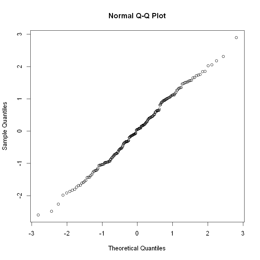
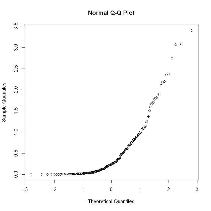
Plot \(x_{(i)}\) vs. \(e_i\). If \(x_1,...,x_n\) do com from a normal distribution then the points should fall close to a straight line. If the plot shows a certain degree of curvature then notifies this may not be a normal model.

x1 <- rnorm(200) # generate random data from N(0,1)
qqnorm(x1) 
x2 <- rgamma(200, shape=.5) # generate gamma with shape=0.5
qqnorm(x2)

Shapiro-Wilk Test

A formalized way of composing the normal QQ plot by the correlation between \(\{X_{(k)}\}\) and \(\{F_0^{-1}(\tau_k)\}\) where \(F_0 = N(0,1)\)

\(H_0:\) data come from \(N(\mu,\sigma)\) for some \(\mu,\sigma\)
statistic

\[W = \frac{(\sum^n a_ix_{(i)})^2}{\sum^n(x_{(i)}-\bar x)^2}, \text{ where }\begin{bmatrix}a_1\\...\\a_n\end{bmatrix} = k_vV^{-1}\begin{bmatrix}e_1\\...\\e_n\end{bmatrix}\]

where \(V[i,j] = cov(Z_{(i)}, Z_{(j)})\) and \(k_v\) is determined so that \(\sum a_i^2 = 1\).

For larger \(n\), then \(W\) is approximately

\[W^* = \frac{(\sum^n e_ix_{(i)})^2}{\sum_{i=1}^n e_i^2(\sum_{i=1}^n (x_{(i)}-\bar x))^2}\]

shapiro.test(x1)
shapiro.test(x2)

    Shapiro-Wilk normality test

data:  x1
W = 0.99369, p-value = 0.5554





    Shapiro-Wilk normality test

data:  x2
W = 0.6741, p-value < 2.2e-16