Two Way ANOVA

Extension of One-way ANOVA, a special case of a GLM.
Two factors, each with $\geq 2$ levels.
Uses a maximum of $(G_1-1) + (G_2 - 1) +(G_1-1)(G_2 - 1)$ (individual + interactions)indicator variables

Two types of factors

FIXED effect: data has been gathered from all the levels of the factor that are of interest
Random effect: interest is in all possible levels of factor, but only a random sample of levels is included in the data.

Case Study The Pygmalion Effect

library(Sleuth2)
data = case1302
head(data)
score = data$Score
company = as.factor(data$Company)
treat = as.factor(data$Treat)

A data.frame: 6 × 3
	Company	Treat	Score
	<fct>	<fct>	<dbl>
1	C1	Pygmalion	80.0
2	C1	Control	63.2
3	C1	Control	69.2
4	C2	Pygmalion	83.9
5	C2	Control	63.1
6	C2	Control	81.5

library(ggplot2)
ggplot(data, aes(x=company, y=score, fill=company)) + geom_boxplot()

ggplot(data, aes(x=treat, y=score, fill=treat))+geom_boxplot()

interaction.plot(company, treat, score, col=c('blue','red'))

interaction.plot(treat, company, score, col=c('blue','red','green','purple','black'))

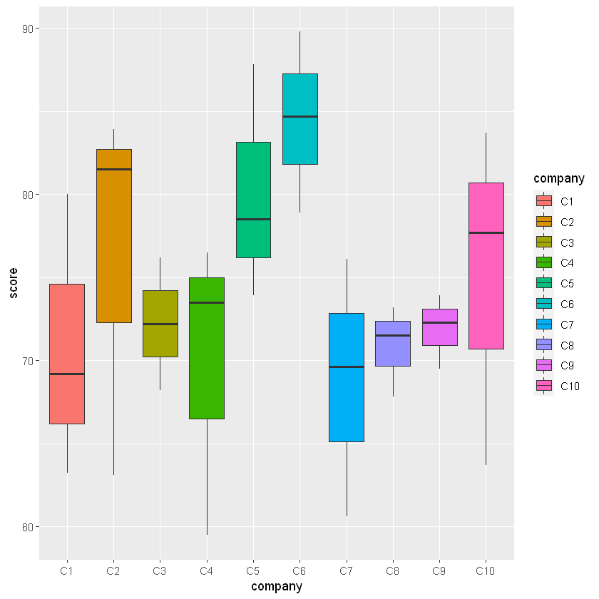
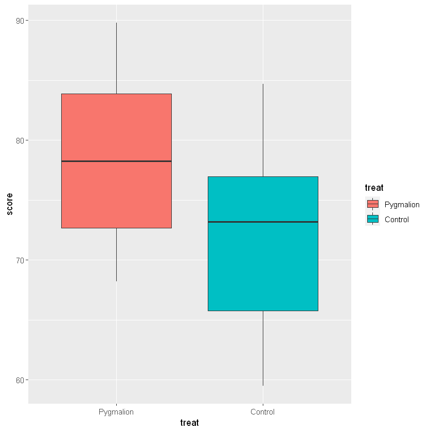
Response: score on a test
Factors:
1. Company: 10 levels (C1,...,C10)
2. Treatment: 2 levels (Pygmalion, Control)
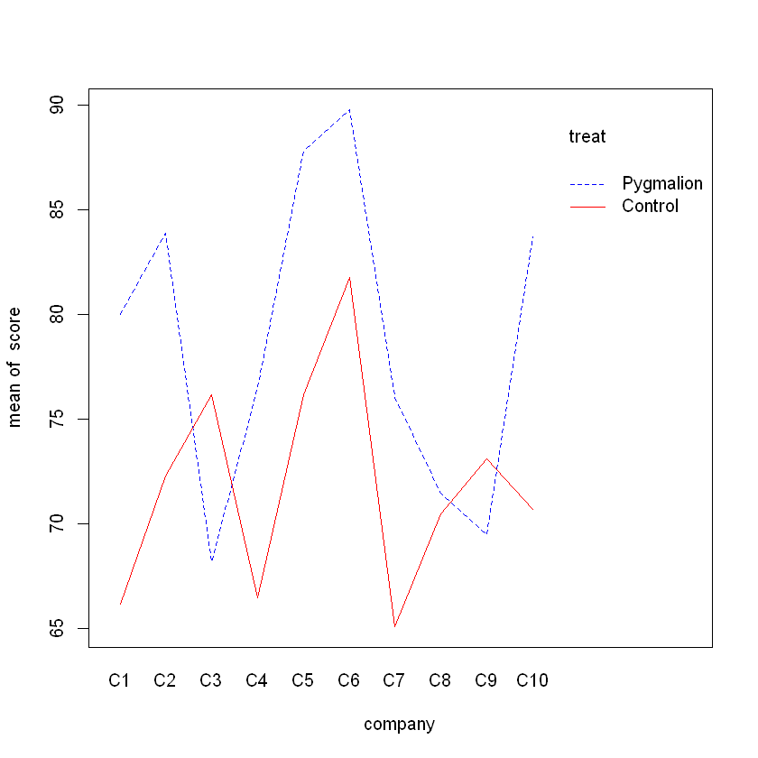
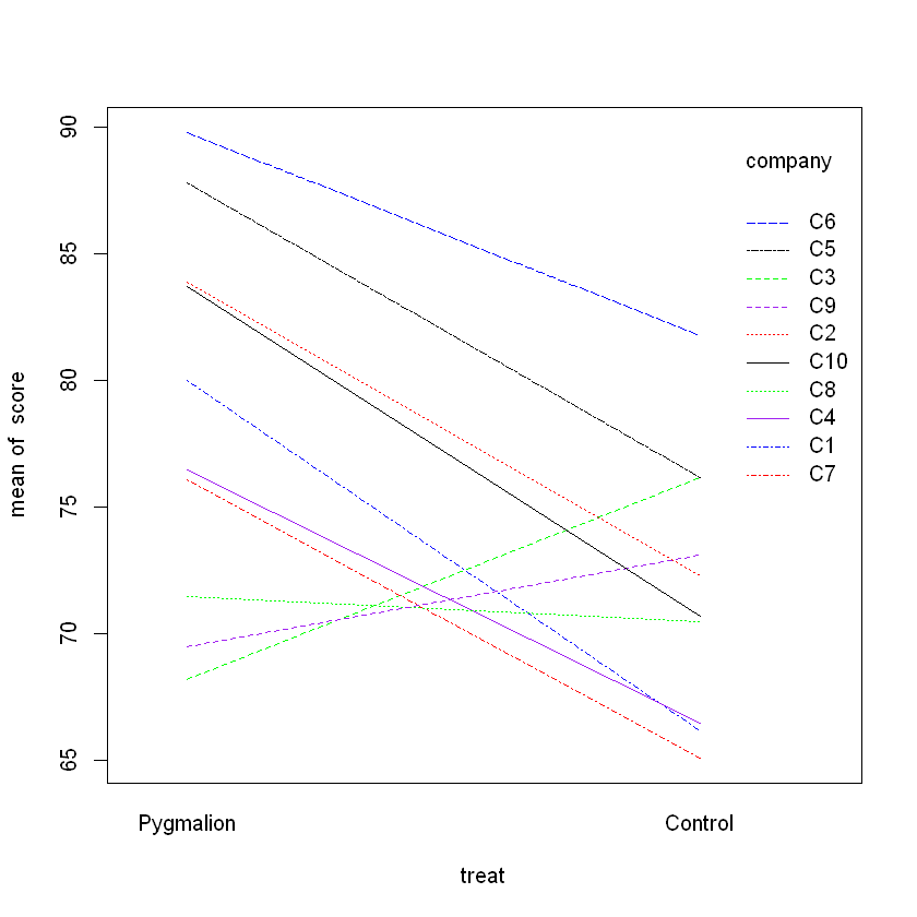
Aim: investigate the interaction between Company and Treatment
Method: Fit a Two-Way ANOVA

Variables

$Y_i$ score for $i$th platoon
Explanatory: $9(\mathbb{I}_{C_m, i})+1(\mathbb{I}_{P_n,i})+9(Interaction)$
For each indicter: $\mathbb{I_{C_m,i}}=I$(ith platoon is from Company m), $\mathbb{I_{P_n,i}}=I$(ith platoon is 'Pygmalion')

Overall test and Partial Test

Overall test $H_0: \beta = \vec{0}$
Partial test $H_0: $ subset of $\beta$ are $0$
Test statistic:

\[\begin{align*} F &= \frac{(SSReg_{\text{full}} - SSReg_{\text{reduced}}) / d.f._{\text{reduced}}} {MSE_{\text{full}}}\\ &= \frac{(RSS_{\text{full}} - RSS_{\text{reduced}}) / d.f._{\text{reduced}}} {MSE_{\text{full}}} \\ &\sim F_{d.f._{\text{full}}, d.f._{\text{error}}} \end{align*}\]

We can use partial test to see if the interaction terms are needed

Interactive Model

model_i = lm(score~company*treat)
summary(model_i)

Call:
lm(formula = score ~ company * treat)

Residuals:
   Min     1Q Median     3Q    Max 
  -9.2   -2.3    0.0    2.3    9.2

Coefficients:
                        Estimate Std. Error t value Pr(>|t|)    
(Intercept)               80.000      7.204  11.105 1.49e-06 ***
companyC2                  3.900     10.188   0.383    0.711    
companyC3                -11.800     10.188  -1.158    0.277    
companyC4                 -3.500     10.188  -0.344    0.739    
companyC5                  7.800     10.188   0.766    0.463    
companyC6                  9.800     10.188   0.962    0.361    
companyC7                 -3.900     10.188  -0.383    0.711    
companyC8                 -8.500     10.188  -0.834    0.426    
companyC9                -10.500     10.188  -1.031    0.330    
companyC10                 3.700     10.188   0.363    0.725    
treatControl             -13.800      8.823  -1.564    0.152    
companyC2:treatControl     2.200     12.477   0.176    0.864    
companyC3:treatControl    21.800     13.477   1.618    0.140    
companyC4:treatControl     3.800     12.477   0.305    0.768    
companyC5:treatControl     2.200     12.477   0.176    0.864    
companyC6:treatControl     5.800     12.477   0.465    0.653    
companyC7:treatControl     2.800     12.477   0.224    0.827    
companyC8:treatControl    12.800     12.477   1.026    0.332    
companyC9:treatControl    17.400     12.477   1.395    0.197    
companyC10:treatControl    0.800     12.477   0.064    0.950    
---
Signif. codes:  0 '***' 0.001 '**' 0.01 '*' 0.05 '.' 0.1 ' ' 1

Residual standard error: 7.204 on 9 degrees of freedom
Multiple R-squared:  0.7388,    Adjusted R-squared:  0.1875 
F-statistic:  1.34 on 19 and 9 DF,  p-value: 0.3358

anova(model_i)

A anova: 4 × 5
	Df	Sum Sq	Mean Sq	F value	Pr(>F)
	<int>	<dbl>	<dbl>	<dbl>	<dbl>
company	9	670.9755	74.55284	1.4366558	0.29901878
treat	1	338.8828	338.88279	6.5303739	0.03091657
company:treat	9	311.4640	34.60711	0.6668895	0.72211538
Residuals	9	467.0399	51.89332	NA	NA

plot(model_i, which=1:2)

Warning message:
"not plotting observations with leverage one:
  1, 4, 7, 8, 9, 12, 15, 18, 21, 24, 27"

Additive Model

model_a = lm(score~company+treat)
summary(model_a)

Call:
lm(formula = score ~ company + treat)

Residuals:
    Min      1Q  Median      3Q     Max 
-10.660  -4.147   1.853   3.853   7.740

Coefficients:
             Estimate Std. Error t value Pr(>|t|)    
(Intercept)  75.61367    4.16822  18.141 5.16e-13 ***
companyC2     5.36667    5.36968   0.999   0.3308    
companyC3     0.19658    6.01886   0.033   0.9743    
companyC4    -0.96667    5.36968  -0.180   0.8591    
companyC5     9.26667    5.36968   1.726   0.1015    
companyC6    13.66667    5.36968   2.545   0.0203 *  
companyC7    -2.03333    5.36968  -0.379   0.7094    
companyC8     0.03333    5.36968   0.006   0.9951    
companyC9     1.10000    5.36968   0.205   0.8400    
companyC10    4.23333    5.36968   0.788   0.4407    
treatControl -7.22051    2.57951  -2.799   0.0119 *  
---
Signif. codes:  0 '***' 0.001 '**' 0.01 '*' 0.05 '.' 0.1 ' ' 1

Residual standard error: 6.576 on 18 degrees of freedom
Multiple R-squared:  0.5647,    Adjusted R-squared:  0.3228 
F-statistic: 2.335 on 10 and 18 DF,  p-value: 0.0564

Partial F test (ANOVA)

Test $H_0:\beta_1 = 0$ (treat Control), $H_a:\beta_1\neq 1$
(T-test or partial F test) $F\sim F_{1, 18}$
$p=0.0119$

Test $H_0: \beta_2=...=\beta_{10} = 0$, $H_a: $ at least one of $\beta_2,...,\beta_{10} \neq 0$
$F\sim F_{9,18}$

anova(model_a)

A anova: 3 × 5
	Df	Sum Sq	Mean Sq	F value	Pr(>F)
	<int>	<dbl>	<dbl>	<dbl>	<dbl>
company	9	670.9755	74.55284	1.723756	0.15556403
treat	1	338.8828	338.88279	7.835401	0.01185757
Residuals	18	778.5039	43.25022	NA	NA

Confidence Interval for two sample t test

\[(\bar{x}_1-\bar{x_2}\pm t\cdot s_p \sqrt{n_1^{-1}+n_2^{-1}} )\]

Least square CI

\[\hat{\beta}_1 \pm t\cdot se(\hat\beta_1)\]

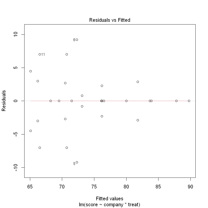
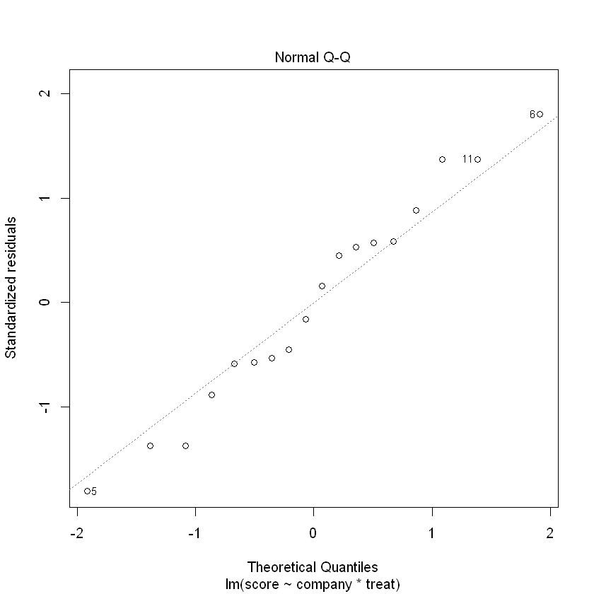
Model Checking

Model is appropriate (include relevant or exclude irrelevant factors)
No outliers
Normality

par(mfrow=c(2,2))
plot(model_a)

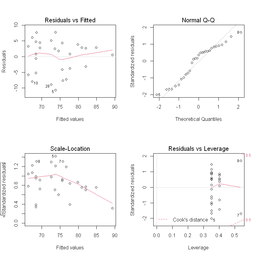
Variance assumption may not be satisfied (variance is decreasing), consider weighted least square regression
Normality satisfied, no dramatic pattern
No outliers