One Way ANOVA

# import data
library(Sleuth2)
percent = case0502$Percent
judge = case0502$Judge

# plot the data
plot(judge, percent)

summary(percent)

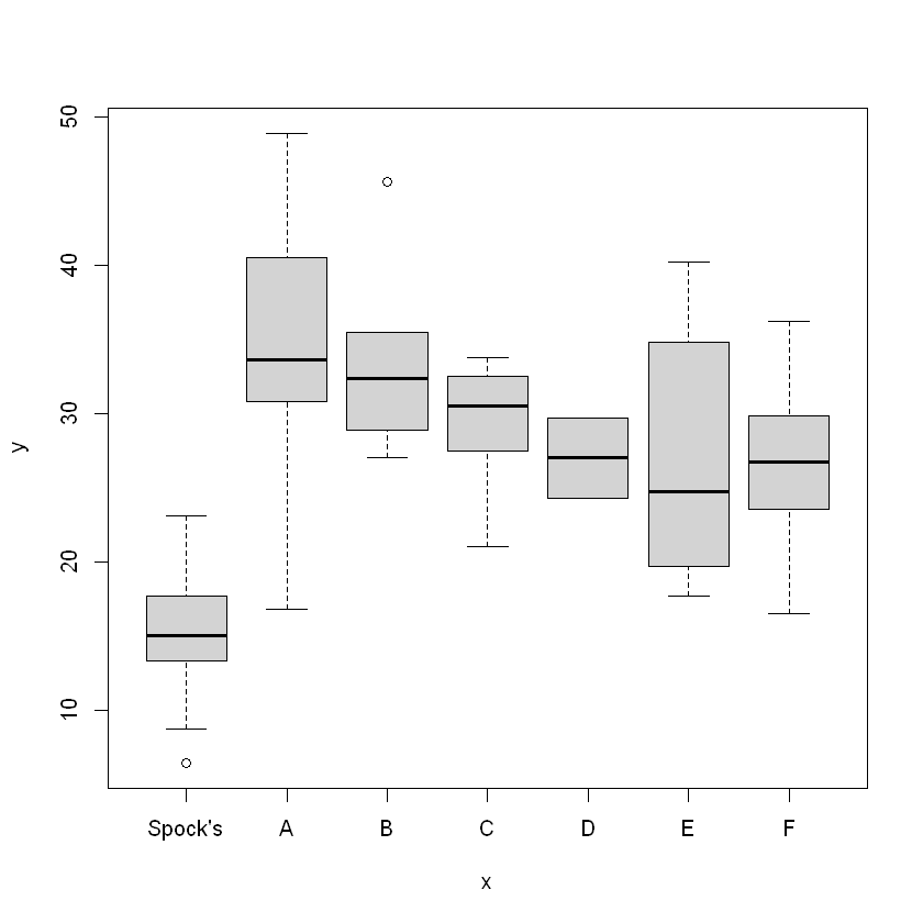
   Min. 1st Qu.  Median    Mean 3rd Qu.    Max. 
   6.40   19.95   27.50   26.58   32.38   48.90

boxplot(percent, horizontal = T)

This looks to be normal, based on Mean vs. Median, and the IQR

t.test(percent, mu = 50)

    One Sample t-test

data:  percent
t = -17.303, df = 45, p-value < 2.2e-16
alternative hypothesis: true mean is not equal to 50
95 percent confidence interval:
 23.85675 29.30847
sample estimates:
mean of x 
 26.58261

One sample two sided test

hypothesis: $H_0:\mu=50$
test statistic: $\frac{\bar{X}-\mu_0}{S/\sqrt{n}}\sim T_{n-1}$
The result is significant, we can reject the hypothesis.

par(mfrow = c(1,2))
hist(percent)
qqnorm(percent)
qqline(percent)

Normality Check

shapiro.test(percent)

    Shapiro-Wilk normality test

data:  percent
W = 0.98763, p-value = 0.9013

$H_0$: data is normal
Test statistics: 0.98763
Probability: 0.9013 is larger
We have evidence that data is normal.

Consider two-sided t-test

Two Sample t-test

groupS <- percent[judge == "Spock's"]
groupS

 6.40000009536743
 8.69999980926514
 13.3000001907349
 13.6000003814697
 15
 15.1999998092651
 17.7000007629395
 18.6000003814697
 23.1000003814697

groupNS <- percent[judge != "Spock's"]
groupNS

 16.7999992370605
 30.7999992370605
 33.5999984741211
 40.5
 48.9000015258789
 27
 28.8999996185303
 32
 32.7000007629395
 35.5
 45.5999984741211
 21
 23.3999996185303
 27.5
 27.5
 30.5
 31.8999996185303
 32.5
 33.7999992370605
 33.7999992370605
 24.2999992370605
 29.7000007629395
 17.7000007629395
 19.7000007629395
 21.5
 27.8999996185303
 34.7999992370605
 40.2000007629395
 16.5
 20.7000007629395
 23.5
 26.3999996185303
 26.7000007629395
 29.5
 29.7999992370605
 31.8999996185303
 36.2000007629395

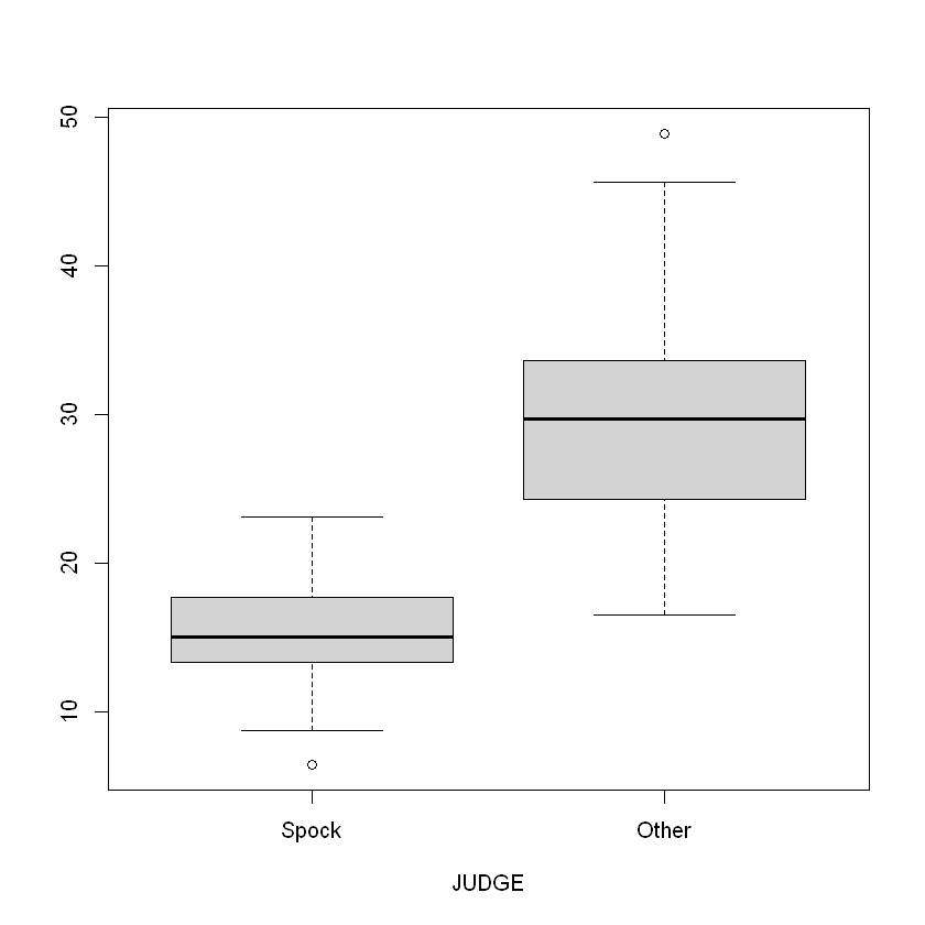
boxplot(groupS, groupNS, xlab="JUDGE", names = c("Spock", "Other"))

Purpose to compare two population means
$H_0$: $\mu_x-\mu_y = D_0 (\text{ commonly }D_0=0)$
Assumptions - two samples are iid from approximately Normal populations - Two samples are independent of each other

Test statistic $t = \frac{(\bar{x}-\bar{y})-D_0}{se(\bar{x}-\bar{y})}$
$$ \begin{align} var(\bar{x}-\bar{y}) &= var(\bar{x}) + var(-\bar{y}) = \sigma_x^2/n_x + (-1)^2\sigma_y^2/n_y \ se(\bar{x}-\bar{y}) &= \sqrt{\sigma_x^2/n_x + \sigma_y^2/x_y} \end{align}$$

Check equal variance assumption

var(groupS)
var(groupNS)
max(var(groupS), var(groupNS)) / min(var(groupS), var(groupNS)) # Rule of Thumb
max(sd(groupS), sd(groupNS)) / min(sd(groupS), sd(groupNS))

 25.3894461176131
 55.2163209681473
 2.17477453869475
 1.47471167985296

Rule of thumb test
$H_0: \sigma_x^2 = \sigma_y^2$
Test statistic: $S_{max}^2 / S^2_{min} = $ larger sample variance / smaller sample variance.
Reject $H_0$ is test-statistic $ > 4$

Variance Ratio F-test

var.test(groupS, groupNS)

    F test to compare two variances

data:  groupS and groupNS
F = 0.45982, num df = 8, denom df = 36, p-value = 0.2482
alternative hypothesis: true ratio of variances is not equal to 1
95 percent confidence interval:
 0.1789822 1.7739665
sample estimates:
ratio of variances 
         0.4598178

Assumptions - Random samples $X_1,X_2$ with size $n_1,n_2$ is drawn from $N(\mu_1,\sigma_1^2), N(\mu_2, \sigma_2^2)$ - $X_1,X_2$ are independent. - Samples size are large (better when samples size are equal)

Test statistic $F = S_1^2/S_2^2 \sim F_{n_1-1,n_2-1}$

$p = 0.07668 > 0.05$, we don't reject the null hypothesis, evidence of equal variance

Two-sample t-test (Satterwaite approximation)

t.test(groupS, groupNS, var.equal = F)

    Welch Two Sample t-test

data:  groupS and groupNS
t = -7.1597, df = 17.608, p-value = 1.303e-06
alternative hypothesis: true difference in means is not equal to 0
95 percent confidence interval:
 -19.23999 -10.49935
sample estimates:
mean of x mean of y 
 14.62222  29.49189

Used when population variance can't be assume to be equal
Test statistic $t = \frac{(\bar{x}-\bar{y}-D_0)}{\sqrt{s^2_x/n_x + s_y^2/n_y}}\sim t_v$, $v = \frac{(s^2_x/n_x + s_y^2/n_y)^2}{(s_x^2/n_x)^2/(n_x-1) + (s_y^2/n_y)^2/(n_y-1)}$. $v$ is calculated by Satterhwaite approximation, round down to the nearest integer

Pooled two-sample t-test

t.test(groupS, groupNS, var.equal = T)

    Two Sample t-test

data:  groupS and groupNS
t = -5.6697, df = 44, p-value = 1.03e-06
alternative hypothesis: true difference in means is not equal to 0
95 percent confidence interval:
 -20.155294  -9.584045
sample estimates:
mean of x mean of y 
 14.62222  29.49189

Assumption population variance are equal
Estimate pooled variance $s_p^2 = \frac{(n_x-1)^2 s_x^2 + (n_y-1)^2 s_y^2}{n_x+n_y-2}$
Test statistic $t = \frac{(\bar{x}-\bar{y})-D_0}{\sqrt{s_p^2(n_x^{-1}+n_y^{-1})}}\sim t_{n_x+n_y-2}$

Based on the tests, we can reject the hypothesis that two samples have the same means
Conclusion Evidence that the percentage of women differs in the two groups

Paired t-test
Requirement $n_x = n_y$, independent samples

Pooled t-test (Left tailed)

$H_0: \mu_x - \mu_y = 0, H_a: \mu_x < \mu_y$

t.test(groupS, groupNS, alternative="less", var.equal= T)

    Two Sample t-test

data:  groupS and groupNS
t = -5.6697, df = 44, p-value = 5.148e-07
alternative hypothesis: true difference in means is less than 0
95 percent confidence interval:
    -Inf -10.463
sample estimates:
mean of x mean of y 
 14.62222  29.49189

Dummy Variable (SLR)

X <- c(rep(1, length(groupS)), rep(0, length(groupNS)))
model <- lm(percent~X)
summary(model)

Call:
lm(formula = percent ~ X)

Residuals:
     Min       1Q   Median       3Q      Max 
-12.9919  -4.6669   0.2581   3.7854  19.4081

Coefficients:
            Estimate Std. Error t value Pr(>|t|)    
(Intercept)   29.492      1.160   25.42  < 2e-16 ***
X            -14.870      2.623   -5.67 1.03e-06 ***
---
Signif. codes:  0 '***' 0.001 '**' 0.01 '*' 0.05 '.' 0.1 ' ' 1

Residual standard error: 7.056 on 44 degrees of freedom
Multiple R-squared:  0.4222,    Adjusted R-squared:  0.409 
F-statistic: 32.15 on 1 and 44 DF,  p-value: 1.03e-06

Model $Y_i=\beta_0+\beta_1X_i+\epsilon_i$, where $X_i=\mathbb{I}(\text{ith observation is from group A})$.
Assumptions - The linear model is appropriate - Gauss-Markov assumptions ($E(\epsilon_i)=0, var(\epsilon_i)=\sigma^2$: Uncorrelated errors) - $\epsilon_i\sim N(0, \sigma^2)$

$H_0:\beta_1 = 0$
Test statistic $t = \frac{b_1}{se(b_1)}\sim t_{N-2}$, $N = n_A + n_{A^c} $

Regression diagnostics

yhats = fitted(model)
errors = residuals(model)
par(mfrow=c(3,2))

hist(errors, xlab="Residuals", breaks = 5)

plot(errors)
abline(0, 0)

plot(model)

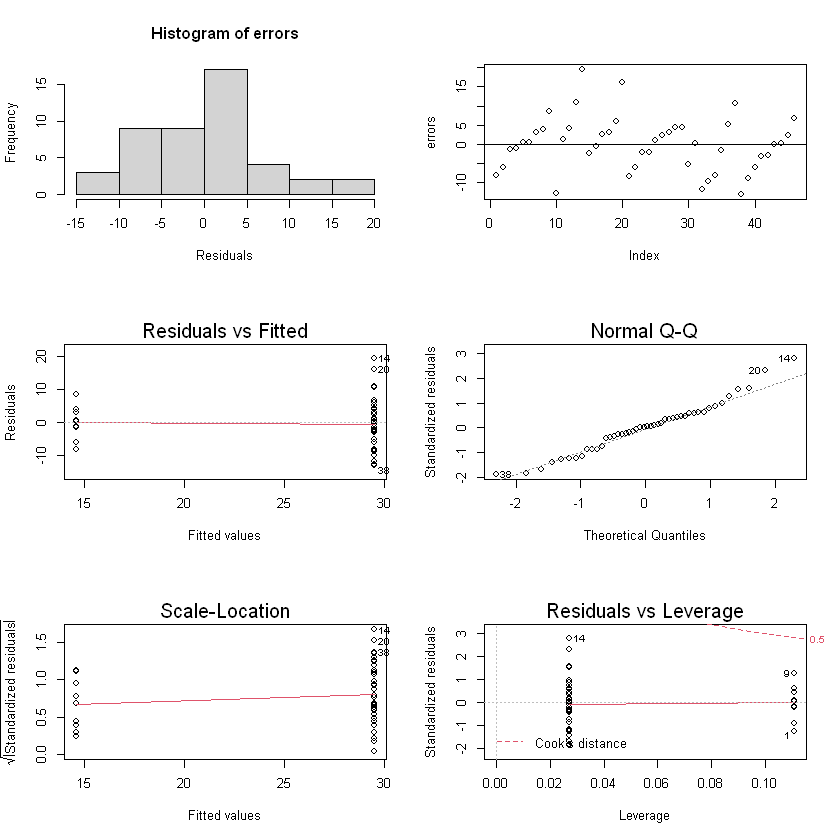
Check Assumptions - Normality: looks like a little bit right skewed (but they might just be outliers) - Constant variance: yes - $E(\epsilon) = 0$: yes

anova(model)

A anova: 2 × 5
	Df	Sum Sq	Mean Sq	F value	Pr(>F)
	<int>	<dbl>	<dbl>	<dbl>	<dbl>
X	1	1600.623	1600.62290	32.14538	1.029666e-06
Residuals	44	2190.903	49.79325	NA	NA

ANOVA for linear regression

$H_0:\beta_1 = 0$
$F=MSR/MSE\sim F_{d.f.variables,\: d.f.errors}$