Binomial Logistic Regression
Y ~ Binomial(m, π)
\(P(Y=y)={m\choose y} \pi^y (1-\pi)^{m-y}\) v.s. Bernoulli => \(\pi\) remains the same in binomial, while in Bernoulli case it is independent for each \(X_i\)
\(E(Y)=m\pi\), \(var(Y)=m\pi(1-\pi)\)
Consider modelling \(Y.m\) be the proportion of success out of \(m\) independent Bernoulli trials \(E(Y/m)=\pi, var(Y/m)=\pi(1-\pi)/m\)
library(Sleuth3)
library(ggplot2)
krunnit = case2101

Extinct = krunnit$Extinct # number of "success"
AtRisk = krunnit$AtRisk
Area = krunnit$Area

pis = Extinct/AtRisk
NExtinct = AtRisk - Extinct # number of "failure"
logitpi = log(pis/(1-(pis)))
logarea = log(Area)
case2101
| Island | Area | AtRisk | Extinct |
|---|---|---|---|
| <fct> | <dbl> | <int> | <int> |
| Ulkokrunni | 185.80 | 75 | 5 |
| Maakrunni | 105.80 | 67 | 3 |
| Ristikari | 30.70 | 66 | 10 |
| Isonkivenletto | 8.50 | 51 | 6 |
| Hietakraasukka | 4.80 | 28 | 3 |
| Kraasukka | 4.50 | 20 | 4 |
| Lansiletto | 4.30 | 43 | 8 |
| Pihlajakari | 3.60 | 31 | 3 |
| Tyni | 2.60 | 28 | 5 |
| Tasasenletto | 1.70 | 32 | 6 |
| Raiska | 1.20 | 30 | 8 |
| Pohjanletto | 0.70 | 20 | 2 |
| Toro | 0.70 | 31 | 9 |
| Luusiletto | 0.60 | 16 | 5 |
| Vatunginletto | 0.40 | 15 | 7 |
| Vatunginnokka | 0.30 | 33 | 8 |
| Tiirakari | 0.20 | 40 | 13 |
| Ristikarenletto | 0.07 | 6 | 3 |
Let \(\pi_i\) be the probability of extinction for each island, assume that this is the same for each species for bird on a particular island
Assume species survival is independent.
Then \(Y_i\sim Binomial(m_i,\pi_i)\)
Unlike binary logistic model for Bernoulli distribution, we can estimate \(\pi_i\) from the data.
Observed response proportion \(\bar{\pi_i} = y_i/m_i\)
Observed or empirical logits: (S-"saturated)


Then the proposed model is based on plot
# cbind(Extinct, NExtinct ~ log(Area) is the way to represent it in R
fitbl <- glm(cbind(Extinct, NExtinct)~log(Area), family=binomial, data=krunnit)
summary(fitbl)
Call:
glm(formula = cbind(Extinct, NExtinct) ~ log(Area), family = binomial,
    data = krunnit)

Deviance Residuals:
     Min        1Q    Median        3Q       Max
-1.71726  -0.67722   0.09726   0.48365   1.49545

Coefficients:
            Estimate Std. Error z value Pr(>|z|)
(Intercept) -1.19620    0.11845 -10.099  < 2e-16 ***
log(Area)   -0.29710    0.05485  -5.416 6.08e-08 ***
---
Signif. codes:  0 '***' 0.001 '**' 0.01 '*' 0.05 '.' 0.1 ' ' 1

(Dispersion parameter for binomial family taken to be 1)

    Null deviance: 45.338  on 17  degrees of freedom
Residual deviance: 12.062  on 16  degrees of freedom
AIC: 75.394

Number of Fisher Scoring iterations: 4
| Df | Deviance | Resid. Df | Resid. Dev | Pr(>Chi) | |
|---|---|---|---|---|---|
| <int> | <dbl> | <int> | <dbl> | <dbl> | |
| NULL | NA | NA | 17 | 45.33802 | NA |
| log(Area) | 1 | 33.27651 | 16 | 12.06151 | 7.994246e-09 |
| (Intercept) | log(Area) | |
|---|---|---|
| (Intercept) | 0.014029452 | -0.002602237 |
| log(Area) | -0.002602237 | 0.003008830 |
| bhat | 2.5 % | 97.5 % | |
|---|---|---|---|
| (Intercept) | -1.1961955 | -1.4283454 | -0.9640456 |
| log(Area) | -0.2971037 | -0.4046132 | -0.1895942 |
Model summary
# observations: 18
# coefficients: 2
fitted model \(logit(\hat\pi) = -1.196-0.297\log(Area)\)
Wald procedures still work the same
\(H_0:\beta_1=0\)
\(z=\frac{\hat\beta_1}{se(\hat\beta_1)}\sim N(0,1)\)
CI: \(\hat\beta_1\pm t_{\alpha,1}se(\hat\beta_1)\)
Interpretation of beta1
Model:
CHanging \(x\) by a factor of \(h\) will change the odds by a multiplicative factor of \(h^{\beta_1}\)
Example: Halving island area changes odds by a factor of \(0.5^{-0.2971} = 1.23\)
Therefore, the odds of extinction on a smaller island are 123% of the odds of extinction on an island double its size.
Halving of area is associated with an increase in the odds of extinction by an estimated 23%. An approximate 95% confidence interval for the percentage change in odds is 14%-32%
| bhat | 2.5 % | 97.5 % | |
|---|---|---|---|
| (Intercept) | 2.291346 | 2.691379 | 1.950773 |
| log(Area) | 1.228675 | 1.323734 | 1.140443 |
| 1 | 2 | 3 | 4 | 5 | 6 | 7 | 8 | 9 | 10 | 11 | 12 | 13 | 14 | 15 | 16 | 17 | 18 | |
|---|---|---|---|---|---|---|---|---|---|---|---|---|---|---|---|---|---|---|
| Extinct | 5.00000 | 3.00000 | 10.00000 | 6.0000 | 3.0000 | 4.000 | 8.0000 | 3.00000 | 5.0000 | 6.0000 | 8.0000 | 2.0000 | 9.0000 | 5.0000 | 7.0000 | 8.0000 | 13.0000 | 3.0000 |
| NExtinct | 70.00000 | 64.00000 | 56.00000 | 45.0000 | 25.0000 | 16.000 | 35.0000 | 28.00000 | 23.0000 | 26.0000 | 22.0000 | 18.0000 | 22.0000 | 11.0000 | 8.0000 | 25.0000 | 27.0000 | 3.0000 |
| pis | 0.06667 | 0.04478 | 0.15152 | 0.1176 | 0.1071 | 0.200 | 0.1860 | 0.09677 | 0.1786 | 0.1875 | 0.2667 | 0.1000 | 0.2903 | 0.3125 | 0.4667 | 0.2424 | 0.3250 | 0.5000 |
| phats | 0.06017 | 0.07036 | 0.09854 | 0.1380 | 0.1595 | 0.162 | 0.1639 | 0.17125 | 0.1854 | 0.2052 | 0.2226 | 0.2516 | 0.2516 | 0.2603 | 0.2842 | 0.3019 | 0.3278 | 0.3998 |
Question: estimate the probability of extinction for a species on the Ulkokrunni island (Area \(= 185.5 km^2\))
\(logit(\hat\pi_{M,1}=)-1.196 - 0.297\log(185.5) = -2.75\)
\(\hat\pi_{M,1} = 0.06\)
logit_result = -1.196 - 0.297 * log(185.5)
pi_m1 = exp(logit_result) / (1+ exp(logit_result))
print(logit_result)
print(pi_m1)
[1] -2.747
[1] 0.06024
Diagnostics
Model assumptions
- Underlying probability model is Binomial variance non constant, is a function of the mean
- Observation independent
- The form of the model is correct
- Liner relationship between logits and explanatory variables
- All relevant variables are included, irrelevant ones excluded
- Sample size is large enough for valid inferences
- outliers
Saturated Model
Model that fits exactly with the data
Most general model possible for the data
Consider one explanatory variable, X with \(n\) unique levels for the outcome, \(Y\sim Binomial(m,\pi)\)
Saturated Model as many parameter coefficients as \(n\)
Fitted Model nested within a FULL model, has (p+1) parameters
Null ModelL intercept only
Checking model adequacy: Form of the model - Deviance Goodness of Fit Test
Form of Hypothesis: $H_0: $ reduced model, $H_a: $ Full model
Deviance GOF test compares the fitted model \(M\) to the saturated model \(S\)
Test Statistic:
This is an asymptotic approximation, so it works better if each \(m_i>5\)
Call:
glm(formula = cbind(Extinct, NExtinct) ~ log(Area), family = binomial,
    data = krunnit)

Deviance Residuals:
    Min       1Q   Median       3Q      Max
-1.7173  -0.6772   0.0973   0.4837   1.4954

Coefficients:
            Estimate Std. Error z value Pr(>|z|)
(Intercept)  -1.1962     0.1184  -10.10  < 2e-16 ***
log(Area)    -0.2971     0.0549   -5.42  6.1e-08 ***
---
Signif. codes:  0 '***' 0.001 '**' 0.01 '*' 0.05 '.' 0.1 ' ' 1

(Dispersion parameter for binomial family taken to be 1)

    Null deviance: 45.338  on 17  degrees of freedom
Residual deviance: 12.062  on 16  degrees of freedom
AIC: 75.39

Number of Fisher Scoring iterations: 4
Example Deviance GOF with R-output \(H_0:\) Fitted model \(logit(\pi)~\log(Area)\)
$H_a: $ Saturated model
Test statistic: \(Deviance = 12.062\) (Residual deviance)
Distribution: \(Deviance\sim \chi^2_{18-2}\)
p-value: \(P(\chi^2_{16}\leq 12.062) = 0.74\)
Conclusion: the data are consistent with \(H_0\); the simpler model with linear function of log(Area) is adequate (fit as well as the saturated model)
0.739700862578766
Small deviance leads to larger p-value and vice versa.
Large p-value means: - fitted model is adequate - Test is not powerful enough to detect inadequacies
Small p-value means: - fitted model is not adequate, consider a more complex model with more explanatory variables or higher order terms and so on OR - response distribution is not adequately modeled by the Binomial distribution, OR - There are severe outliers
Outliers
Response (raw) residuals
Standardized residuals
- Pearson Residuals: uses estimate of s.d. of \(Y\)
- Deviance Residuals: defined so that the sum of the square of the residuals is the deviance
# response residuals
rres = residuals(fitbl, type="response")
# pearson residuals
pres = residuals(fitbl, type="pearson")
# Deviance residuals
dres = residuals(fitbl, type="deviance")
cbind(pis, phats, rres, pres, dres)
| pis | phats | rres | pres | dres | |
|---|---|---|---|---|---|
| 1 | 0.06667 | 0.06017 | 0.006493 | 0.23646 | 0.23266 |
| 2 | 0.04478 | 0.07036 | -0.025585 | -0.81883 | -0.87369 |
| 3 | 0.15152 | 0.09854 | 0.052975 | 1.44400 | 1.34958 |
| 4 | 0.11765 | 0.13800 | -0.020351 | -0.42139 | -0.43071 |
| 5 | 0.10714 | 0.15946 | -0.052319 | -0.75619 | -0.79584 |
| 6 | 0.20000 | 0.16205 | 0.037951 | 0.46058 | 0.44746 |
| 7 | 0.18605 | 0.16389 | 0.022155 | 0.39247 | 0.38577 |
| 8 | 0.09677 | 0.17125 | -0.074480 | -1.10075 | -1.18097 |
| 9 | 0.17857 | 0.18542 | -0.006844 | -0.09318 | -0.09363 |
| 10 | 0.18750 | 0.20524 | -0.017742 | -0.24850 | -0.25127 |
| 11 | 0.26667 | 0.22264 | 0.044030 | 0.57969 | 0.56727 |
| 12 | 0.10000 | 0.25158 | -0.151576 | -1.56220 | -1.71726 |
| 13 | 0.29032 | 0.25158 | 0.038747 | 0.49717 | 0.48934 |
| 14 | 0.31250 | 0.26030 | 0.052203 | 0.47588 | 0.46659 |
| 15 | 0.46667 | 0.28415 | 0.182515 | 1.56733 | 1.49545 |
| 16 | 0.24242 | 0.30185 | -0.059429 | -0.74367 | -0.75939 |
| 17 | 0.32500 | 0.32783 | -0.002828 | -0.03810 | -0.03813 |
| 18 | 0.50000 | 0.39984 | 0.100157 | 0.50082 | 0.49570 |
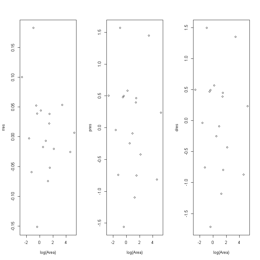
Pearson vs Deviance Residuals
- Both asymptotically to \(N(0,1)\)
- Possible outlier if \(|res|>2\)
- Definite outlier if \(|res|>3\)
- Under small \(n\) \(D_{res}\) closer to \(N(0,1)\) then \(P_{res}\)
- When \(\hat\pi\) close to extreme (0, 1), \(P_{res}\) are unstable
Problems and Solutions
Issues Related to General Linear Models
extrapolation
- Don't make inferences/predictions outside range of observed data
- Model may no longer be appropriate
Multicollinearity
Consequences includes
- unstable fitted equation
- Coefficient that should be statistically significant while not
- Coefficient may have wrong sign
- Sometimes large \(se(\beta)\)
- Sometimes numerical procedure to find MLEs does not converge
Influential Points
Model: overfit issue, should build model on training data (cross validation)
Problems specific to Logistic Regression
Extra-binomial variation (over dispersion) - variance of \(Y_i\) greater than \(m_i\pi_i(1-\pi_i)\) - Does not bias \(\hat\beta\)'s but se of \(\hat\beta\)'s will be too small
Solution: add one more parameter to the model, \(\phi\)-dispersion parameter. Then \(var(Y_i)=\phi m_i\pi_i(1-\pi_i)\)
Complete separation
- One or a linear combination of explanatory variables perfectly predict whether \(Y=1\lor 0\)
- In Binary response, when \(y_i=1,\hat y_i=1\), then \(\sum_{i=1}^n\{y_i\log(\hat y_i + (1-y_i)\log(1-\hat y_i))=0\}\)
- MLE cannot be computed
Quasi-complete separation:
- explanatory variables predict \(Y=1\lor 0\) almost perfectly
- MLE are numerically unstable
Solution: simplify the model. Try other methods like penalized maximum likelihood, exact logistic regression, Bayesian methods
Conclusions about Logistic Regression
False Logistic regression describes population proportion of probability as a linear function of explanatory variables.
Non-linear \(\hat\pi = e^{\hat\mu}/(1+e^{\hat\mu})\)
Hence Logistic regression is a nonlinear regression model
Extra-binomial variation
Suppose \(X_1,...,X_m\) are not independent but identically distributed \(\sim Bernoulli(\pi)\). Further suppose \(\forall X_i,X_j. cov(X_1,X_j)=\rho, \rho>0\).
Let \(Y_1=\sum_i^{m_1}X_i\)
Then
Therefore, the model for variance:
estimate of \(\hat\psi\) by scaled Pearson chi-square statistic
\(\hat\psi>>1\) indicates evidence of over-dispersion
\(\psi\) does not effect \(E(Y_i)\), hence using over-dispersion does not change \(\hat\beta\)
The standard errors under this assumption is \(se_{\psi}(\hat\beta)=\sqrt{\hat\psi}se(\hat\beta)\)
The following two ways are equivalent
# manually conpute the psi hat
psihat = sum(residuals(fitbl, type="pearson")^2/fitbl$df.residual)
psihat
0.73257293737338
Call:
glm(formula = cbind(Extinct, NExtinct) ~ log(Area), family = binomial,
    data = krunnit)

Deviance Residuals:
    Min       1Q   Median       3Q      Max
-1.7173  -0.6772   0.0973   0.4837   1.4954

Coefficients:
            Estimate Std. Error z value Pr(>|z|)
(Intercept)  -1.1962     0.1014  -11.80  < 2e-16 ***
log(Area)    -0.2971     0.0469   -6.33  2.5e-10 ***
---
Signif. codes:  0 '***' 0.001 '**' 0.01 '*' 0.05 '.' 0.1 ' ' 1

(Dispersion parameter for binomial family taken to be 0.7326)

    Null deviance: 45.338  on 17  degrees of freedom
Residual deviance: 12.062  on 16  degrees of freedom
AIC: 75.39

Number of Fisher Scoring iterations: 4
# use quasi binomial family
fitbl2 <- glm(cbind(Extinct, NExtinct)~log(Area), family=quasibinomial, data=krunnit)
fitbl2
Call:  glm(formula = cbind(Extinct, NExtinct) ~ log(Area), family = quasibinomial,
    data = krunnit)

Coefficients:
(Intercept)    log(Area)
     -1.196       -0.297

Degrees of Freedom: 17 Total (i.e. Null);  16 Residual
Null Deviance:      45.3
Residual Deviance: 12.1     AIC: NA
Using Logistic Regression for Classification
Want: \(y^*\mid (x_1^*, ...,x_p^*)= \mathbb{I}\)
Do: calculate \(\hat\pi_M^*\) be the estimated probability that \(y^*=1\) based on the fitted model given \(X_i=x_i^*\), then predict that \(y^* = \mathbb{I}(\hat\pi_M^* \text{is large enough})\)
Need: a good cutoff \(\hat\pi_M^*\)
Classification
Try different cutoffs and see which gives fewest incorrect classifications
- Useful if proportion of 1's and 0's in date reflect their relative proportions in the population
- Likely to overestimate. To overcome,cross-validation (training group vs. validation group)
Confusion Matrix
https://en.wikipedia.org/wiki/Confusion_matrix
Choose a cutoff probability based on one of the 5 criteria for success of classification that is most important to you
Examples
- High sensitivity makes good screening test
- High specificity makes a good confirmatory test
- A screening test followed by a confirmatory test is good (but expensive) diagnostic procedure