Binary logistic regression

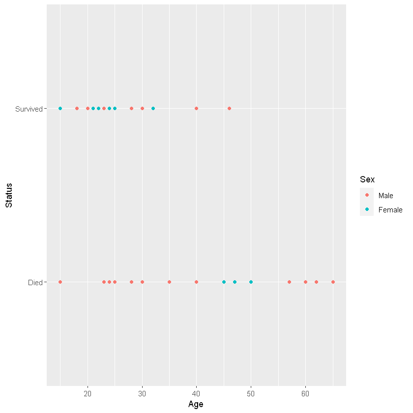
Case Study: Donner Party

library(Sleuth2)
donner = case2001
Age = donner$Age
Sex = donner$Sex
Status = donner$Status

# contingency table
xtabs(~Status+Sex, data=donner)

          Sex
Status     Male Female
  Died       20      5
  Survived   10     10

summary(Age)

   Min. 1st Qu.  Median    Mean 3rd Qu.    Max. 
   15.0    24.0    28.0    31.8    40.0    65.0

Response \(Y_i=\{0,1\}\) survived or died
Predictor: \(X_i\) age/sex

Model

\(Y_i\mid X_i=\mathbb{I}\)(response is in category of interest)\(\sim Bernoulli(\pi_i)\)
\(E(Y_i\mid X_i)=\pi_i, var(Y_i\mid X_i)=\pi_1(1-\pi_i)\)

Generalized Linear Models

Having response \(Y\) can a set of explanatory variables \(X_1,...,X_p\)

Want \(E(Y)\) as a linear function in the parameters, ie. \(g(E(Y))=X\beta\)

Key idea: find the link function \(g\) such that the model is true

Some link functions

link	function	usual distribution of \(Y\mid X\)
identity	\(g(\mu)=\mu\)	normal
log	\(g(\mu)=\log\mu,\mu>0\)	Poisson(count data)
logistic	\(g(\mu)=\log(\mu/(1-\mu)),0<\mu<1\)	Bernoulli(binary),Binomial

GLM vs. Transformation

For transformation, transforming \(Y\) so it has an approximate normal distribution with constant variance
For GLM, distribution of \(Y\) not restricted to Normal
Model parameters describe \(g(E(Y))\) rather than \(E(g(Y))\)
GLM provide a unified theory of modeling that encompasses the most important models for continuous and discrete variables

Binary Logistic Regression

Let \(\pi=P("success"),0<\pi<1\)
The odds in favor of success is \(\frac{\pi}{1-\pi}\)
The log odds is \(\log(\frac{\pi}{1-\pi})\)

Model

\(\log(\frac{\pi}{1-\pi}) = \beta_0 + \beta_1X_1+...+\beta_pX_p\)

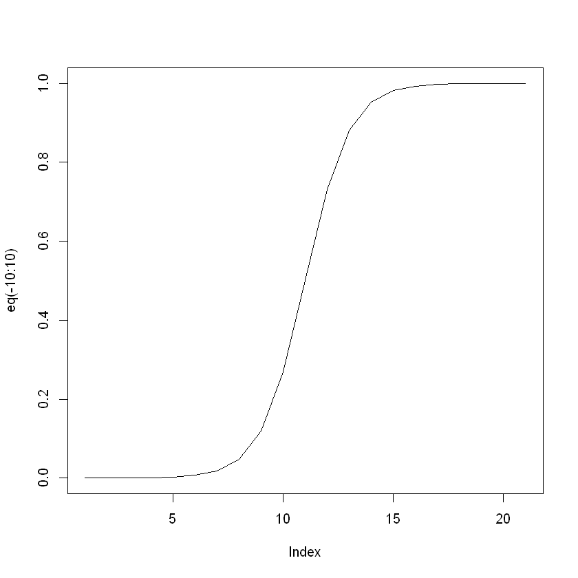
Let the linear predictor \(\eta=\beta_0 + \beta_1X_1+...+\beta_pX_p\), then Logistic function is \(\pi(\eta)=\frac{e^{\eta}}{1+e^\eta}\)

eq <- function(x){exp(x)/(1+exp(x))}
plot(eq(-10:10), type='l')

log-odds \(\log(\frac{\pi}{1-\pi})\in(-\infty, \infty)\), is increasing function.
Predicts the natural log of the odds for a subject bing in one category or another
Regression coefficients can be used to estimate odds ratio for each of the independent variables
Tell which predictors can be used to determine if a subject was in a category of interest

MLE

Date: \(Y_i=\mathbb{I}(\text{if response is in category of interest})\)
Model: \(P(Y_i=y_1)=\pi_i^{y_{i}}(1-\pi_i)^{1-y_{i}}\)
Assumption: The observations are independent.
Joint density:

\[P(Y_1=y_1,...,Y_n=y_n)=\prod_1^n \pi_i^{y_{i}}(1-\pi_i)^{1-y_{i}}\]

\[\pi_i = \frac{\exp(\beta_0+\beta_1X_{i1}+...+\beta_pX_{ip})}{1+\exp(\beta_0+\beta_1X_{i1}+...+\beta_pX_{ip})}\]

Likelihood function: plug in observed data and think of the joint density as a function of \(\beta\)'s

\[\mathcal{L}(\beta_0,...,\beta_p)=\prod_{1^n}\pi_i\vec\beta^{y_i}(1-\pi_i{\vec\beta})^{1-y_i}\]

There is no explicit expression for the max likelihood estimators. Two iterative numerical solution methods are Newton-Raphson algorithm and Fisher scoring or IWLS (In R, glm())

# additive
fita<-glm(Status~Age+Sex, family=binomial, data=donner)
summary(fita)

Call:
glm(formula = Status ~ Age + Sex, family = binomial, data = donner)

Deviance Residuals: 
    Min       1Q   Median       3Q      Max  
-1.7445  -1.0441  -0.3029   0.8877   2.0472

Coefficients:
            Estimate Std. Error z value Pr(>|z|)  
(Intercept)  1.63312    1.11018   1.471   0.1413  
Age         -0.07820    0.03728  -2.097   0.0359 *
SexFemale    1.59729    0.75547   2.114   0.0345 *
---
Signif. codes:  0 '***' 0.001 '**' 0.01 '*' 0.05 '.' 0.1 ' ' 1

(Dispersion parameter for binomial family taken to be 1)

    Null deviance: 61.827  on 44  degrees of freedom
Residual deviance: 51.256  on 42  degrees of freedom
AIC: 57.256

Number of Fisher Scoring iterations: 4

anova(fita)

A anova: 3 × 4
	Df	Deviance	Resid. Df	Resid. Dev
	<int>	<dbl>	<int>	<dbl>
NULL	NA	NA	44	61.82654
Age	1	5.535820	43	56.29072
Sex	1	5.034437	42	51.25628

# modelling "Died"
Status2 = relevel(Status, ref="Survived")
fitad <- glm(Status2 ~ Age + Sex, family=binomial, data=donner)
summary(fitad)

Call:
glm(formula = Status2 ~ Age + Sex, family = binomial, data = donner)

Deviance Residuals: 
    Min       1Q   Median       3Q      Max  
-2.0472  -0.8877   0.3029   1.0441   1.7445

Coefficients:
            Estimate Std. Error z value Pr(>|z|)  
(Intercept) -1.63312    1.11018  -1.471   0.1413  
Age          0.07820    0.03728   2.097   0.0359 *
SexFemale   -1.59729    0.75547  -2.114   0.0345 *
---
Signif. codes:  0 '***' 0.001 '**' 0.01 '*' 0.05 '.' 0.1 ' ' 1

(Dispersion parameter for binomial family taken to be 1)

    Null deviance: 61.827  on 44  degrees of freedom
Residual deviance: 51.256  on 42  degrees of freedom
AIC: 57.256

Number of Fisher Scoring iterations: 4

# Reference group as "Male"
Sex2 = relevel(Sex, ref="Male")
fitadf <- glm(Status2~Age + Sex2, family=binomial, data=donner)
summary(fitadf)

Call:
glm(formula = Status2 ~ Age + Sex2, family = binomial, data = donner)

Deviance Residuals: 
    Min       1Q   Median       3Q      Max  
-2.0472  -0.8877   0.3029   1.0441   1.7445

Coefficients:
            Estimate Std. Error z value Pr(>|z|)  
(Intercept) -1.63312    1.11018  -1.471   0.1413  
Age          0.07820    0.03728   2.097   0.0359 *
Sex2Female  -1.59729    0.75547  -2.114   0.0345 *
---
Signif. codes:  0 '***' 0.001 '**' 0.01 '*' 0.05 '.' 0.1 ' ' 1

(Dispersion parameter for binomial family taken to be 1)

    Null deviance: 61.827  on 44  degrees of freedom
Residual deviance: 51.256  on 42  degrees of freedom
AIC: 57.256

Number of Fisher Scoring iterations: 4

# Additive model for survived
fitasf <- glm(Status~Age + Sex2, family=binomial, data=donner)
summary(fitasf)

Call:
glm(formula = Status ~ Age + Sex2, family = binomial, data = donner)

Deviance Residuals: 
    Min       1Q   Median       3Q      Max  
-1.7445  -1.0441  -0.3029   0.8877   2.0472

Coefficients:
            Estimate Std. Error z value Pr(>|z|)  
(Intercept)  1.63312    1.11018   1.471   0.1413  
Age         -0.07820    0.03728  -2.097   0.0359 *
Sex2Female   1.59729    0.75547   2.114   0.0345 *
---
Signif. codes:  0 '***' 0.001 '**' 0.01 '*' 0.05 '.' 0.1 ' ' 1

(Dispersion parameter for binomial family taken to be 1)

    Null deviance: 61.827  on 44  degrees of freedom
Residual deviance: 51.256  on 42  degrees of freedom
AIC: 57.256

Number of Fisher Scoring iterations: 4

# the order of independent variable does not metter
fitsaf <- glm(Status~ Sex2+Age, family=binomial, data=donner)
summary(fitsaf)

Call:
glm(formula = Status ~ Sex2 + Age, family = binomial, data = donner)

Deviance Residuals: 
    Min       1Q   Median       3Q      Max  
-1.7445  -1.0441  -0.3029   0.8877   2.0472

Coefficients:
            Estimate Std. Error z value Pr(>|z|)  
(Intercept)  1.63312    1.11018   1.471   0.1413  
Sex2Female   1.59729    0.75547   2.114   0.0345 *
Age         -0.07820    0.03728  -2.097   0.0359 *
---
Signif. codes:  0 '***' 0.001 '**' 0.01 '*' 0.05 '.' 0.1 ' ' 1

(Dispersion parameter for binomial family taken to be 1)

    Null deviance: 61.827  on 44  degrees of freedom
Residual deviance: 51.256  on 42  degrees of freedom
AIC: 57.256

Number of Fisher Scoring iterations: 4

anova(fitasf)

A anova: 3 × 4
	Df	Deviance	Resid. Df	Resid. Dev
	<int>	<dbl>	<int>	<dbl>
NULL	NA	NA	44	61.82654
Age	1	5.535820	43	56.29072
Sex2	1	5.034437	42	51.25628

anova(fitsaf)

A anova: 3 × 4
	Df	Deviance	Resid. Df	Resid. Dev
	<int>	<dbl>	<int>	<dbl>
NULL	NA	NA	44	61.82654
Sex2	1	4.540267	43	57.28628
Age	1	6.029991	42	51.25628

# Higher order model with 3 higher order/interaction terms
fitfull <- glm(Status~Age + Sex2 + Age:Sex2+I(Age^2)+I(Age^2):Sex2, family=binomial, data=donner)
summary(fitfull)

Call:
glm(formula = Status ~ Age + Sex2 + Age:Sex2 + I(Age^2) + I(Age^2):Sex2, 
    family = binomial, data = donner)

Deviance Residuals: 
    Min       1Q   Median       3Q      Max  
-2.3396  -0.9757  -0.3438   0.5269   1.5901

Coefficients:
                     Estimate Std. Error z value Pr(>|z|)
(Intercept)         -3.318484   3.940184  -0.842    0.400
Age                  0.183031   0.226632   0.808    0.419
Sex2Female           0.265286  10.455222   0.025    0.980
I(Age^2)            -0.002803   0.002985  -0.939    0.348
Age:Sex2Female       0.299877   0.696050   0.431    0.667
Sex2Female:I(Age^2) -0.007356   0.010689  -0.688    0.491

(Dispersion parameter for binomial family taken to be 1)

    Null deviance: 61.827  on 44  degrees of freedom
Residual deviance: 45.361  on 39  degrees of freedom
AIC: 57.361

Number of Fisher Scoring iterations: 5

# interaction model
fitas <- glm(Status~Age*Sex2, family=binomial,data=donner)
summary(fitas)

Call:
glm(formula = Status ~ Age * Sex2, family = binomial, data = donner)

Deviance Residuals: 
    Min       1Q   Median       3Q      Max  
-2.2279  -0.9388  -0.5550   0.7794   1.6998

Coefficients:
               Estimate Std. Error z value Pr(>|z|)  
(Intercept)     0.31834    1.13103   0.281   0.7784  
Age            -0.03248    0.03527  -0.921   0.3571  
Sex2Female      6.92805    3.39887   2.038   0.0415 *
Age:Sex2Female -0.16160    0.09426  -1.714   0.0865 .
---
Signif. codes:  0 '***' 0.001 '**' 0.01 '*' 0.05 '.' 0.1 ' ' 1

(Dispersion parameter for binomial family taken to be 1)

    Null deviance: 61.827  on 44  degrees of freedom
Residual deviance: 47.346  on 41  degrees of freedom
AIC: 55.346

Number of Fisher Scoring iterations: 5

anova(fitasf, test="Chisq")

A anova: 3 × 5
	Df	Deviance	Resid. Df	Resid. Dev	Pr(>Chi)
	<int>	<dbl>	<int>	<dbl>	<dbl>
NULL	NA	NA	44	61.82654	NA
Age	1	5.535820	43	56.29072	0.01863103
Sex2	1	5.034437	42	51.25628	0.02484816

vcov(fitasf, digits=3)

A matrix: 3 × 3 of type dbl
	(Intercept)	Age	Sex2Female
(Intercept)	1.23250837	-0.038472741	0.06007099
Age	-0.03847274	0.001390134	-0.00823197
Sex2Female	0.06007099	-0.008231970	0.57073339

cbind(bhat=coef(fitasf), confint.default(fitasf)) # CI for beta's

A matrix: 3 × 3 of type dbl
	bhat	2.5 %	97.5 %
(Intercept)	1.63312031	-0.5428002	3.809040837
Age	-0.07820407	-0.1512803	-0.005127799
Sex2Female	1.59729350	0.1166015	3.077985503

exp(coef(fitasf)) # odd ratios

(Intercept) 5.11982524825608
Age         0.924775685984312
Sex2Female  4.93964517580916

exp(cbind(OR=coef(fitasf), confint.default(fitasf))) # Ci for odd ratios

A matrix: 3 × 3 of type dbl
	OR	2.5 %	97.5 %
(Intercept)	5.1198252	0.5811187	45.1071530
Age	0.9247757	0.8596067	0.9948853
Sex2Female	4.9396452	1.1236716	21.7146143

Wald Chi-sq Procedures

logistic regression inference on a single \(\beta\)

Hypotheses: \(H_0:\beta_j=0,H_a:\beta_j\neq 0\)
Test statistic: \(z=\hat\beta_j/se(\hat\beta_j)\), \(\hat\beta_j\) is MLE for \(\beta_j\)
By standard large-sample results, MLE's are normally distributed. Thus, for large \(n\), under \(H_0\), z is an observation from an approx. \(N(0,1)\). Note that \(Z^2\sim \chi_1\), we can use chisq for p-value
95% CI: \(\hat\beta_j \pm 1.96se(\hat\beta_j)\)

Since the logistic function is monotonic, we can expand CI by doing monotonic transformation (e.x. multiplication and exp)

# Wald test
library(aod)
wald.test(Sigma=vcov(fitasf), b=coef(fitasf), Terms=2:3)

Wald test:
----------
Chi-squared test:
X2 = 6.9, df = 2, P(> X2) = 0.032

wald.test(Sigma=vcov(fitas), b=coef(fitas), Terms=4)

Wald test:
----------
Chi-squared test:
X2 = 2.9, df = 1, P(> X2) = 0.086

Model Assumptions

Underlying probability model for response is Bernoulli
Observations are independent
The form of the model is correct
- Linear relationship between logits and explanatory variables
- All relevant variables are included; irrelevant ones excluded
Sample size is large enough for valid inference

B Logistic R vs. Linear R - both utilize MLR's for the \(\beta\)'s - Less assumption to check for than in linear regression - No need to check for outliers - No residual plots - Variance is not constant

Need to test - (designing aspect) Independence of observations - (inference) Form of the model: test higher-order terms such as non-linear in X, interaction, and higher order interaction

Wald cs. LRT test

Walk test on single \(\beta = 0\), LRT find \(k\geq 1\) \(\beta\)'s.
LRT compares nested models
LRT allow small to moderate sample sizes \(\beta\) near boundary of parameter space

Comparing models: Likelihood Ratio Test

Idea: compare likelihood of data under Full model, \(\mathcal{L}_F\) to likelihood under REDUCED model \(\mathcal{L}_R\) of same data. the likelihood ratio \(\mathcal{L}_R/\mathcal{L}F\) where \(\mathcal{L}_R\leq \mathcal{L}_F\)
Hypothesis: \(H_0:\beta_1=...\beta_k=0\) (Reduced model is appropriate, fits data as swll as Full model)\(H_a:\) at least one of betas is not 0 (full model is better)
Test statistic: Deviance (residual)

\[G^2 = -2\log\mathcal{L}_R - (-2\log\mathcal{L}_F)=-2\log(\mathcal{L}_R/\mathcal{L}_F)\sim \chi^2_k\]

For large \(n\), under \(H_0\), \(G^2\) is an observation from a chi-square distribution with \(k\) d.f.

Exercise

Models

\[\begin{align*} log(\frac{\pi_i}{1-\pi_i}) &= \\&(1) a_0+a_1Age_i+a_2I_{Female, i}\\ &(2) \beta_0 +\beta_1Age_i+\beta_2 I_{female_i,i} + \beta_3Age_i*I_{female,i}+\beta_4Age_i^2 + \beta_5Age_i^2*I_{Female, i} \\ &(3) \gamma_0 + \gamma_1Age_i + \gamma_2I_{Female, i} + \gamma_3Age_i *I_{Female, i}\end{align*}\]

# additive model (model 1)
fitadd <- glm(Status~Age + Sex, family=binomial, donner)
summary(fitadd)

Call:
glm(formula = Status ~ Age + Sex, family = binomial, data = donner)

Deviance Residuals: 
    Min       1Q   Median       3Q      Max  
-1.7445  -1.0441  -0.3029   0.8877   2.0472

Coefficients:
            Estimate Std. Error z value Pr(>|z|)  
(Intercept)  1.63312    1.11018   1.471   0.1413  
Age         -0.07820    0.03728  -2.097   0.0359 *
SexFemale    1.59729    0.75547   2.114   0.0345 *
---
Signif. codes:  0 '***' 0.001 '**' 0.01 '*' 0.05 '.' 0.1 ' ' 1

(Dispersion parameter for binomial family taken to be 1)

    Null deviance: 61.827  on 44  degrees of freedom
Residual deviance: 51.256  on 42  degrees of freedom
AIC: 57.256

Number of Fisher Scoring iterations: 4

# full model (model 2)
fitfull <- glm(Status~Age + Sex + Age: Sex + I(Age^2) + I(Age^2):Sex, 
               family=binomial, donner)
summary(fitfull)

Call:
glm(formula = Status ~ Age + Sex + Age:Sex + I(Age^2) + I(Age^2):Sex, 
    family = binomial, data = donner)

Deviance Residuals: 
    Min       1Q   Median       3Q      Max  
-2.3396  -0.9757  -0.3438   0.5269   1.5901

Coefficients:
                    Estimate Std. Error z value Pr(>|z|)
(Intercept)        -3.318484   3.940184  -0.842    0.400
Age                 0.183031   0.226632   0.808    0.419
SexFemale           0.265286  10.455222   0.025    0.980
I(Age^2)           -0.002803   0.002985  -0.939    0.348
Age:SexFemale       0.299877   0.696050   0.431    0.667
SexFemale:I(Age^2) -0.007356   0.010689  -0.688    0.491

(Dispersion parameter for binomial family taken to be 1)

    Null deviance: 61.827  on 44  degrees of freedom
Residual deviance: 45.361  on 39  degrees of freedom
AIC: 57.361

Number of Fisher Scoring iterations: 5

# interative model (model 3)
fitint <- glm(Status~Age*Sex, family=binomial, donner)
summary(fitint)

Call:
glm(formula = Status ~ Age * Sex, family = binomial, data = donner)

Deviance Residuals: 
    Min       1Q   Median       3Q      Max  
-2.2279  -0.9388  -0.5550   0.7794   1.6998

Coefficients:
              Estimate Std. Error z value Pr(>|z|)  
(Intercept)    0.31834    1.13103   0.281   0.7784  
Age           -0.03248    0.03527  -0.921   0.3571  
SexFemale      6.92805    3.39887   2.038   0.0415 *
Age:SexFemale -0.16160    0.09426  -1.714   0.0865 .
---
Signif. codes:  0 '***' 0.001 '**' 0.01 '*' 0.05 '.' 0.1 ' ' 1

(Dispersion parameter for binomial family taken to be 1)

    Null deviance: 61.827  on 44  degrees of freedom
Residual deviance: 47.346  on 41  degrees of freedom
AIC: 55.346

Number of Fisher Scoring iterations: 5

# p-value for model2 vs. model1
1 - pchisq(5.895, 3)

0.11683196297711

Q1

Using R output determine whether a model with the 3 higher order polynomial terms and interaction term is an improvement over the additive model

Higher order interaction vs. additive Hypotheses: \(H_0:\beta_3=\beta_4=\beta_5 = 0\)

Test statistic \(G^2 = 51.256 - 45.361 = 5.895\sim \chi^2_3\)

p-value: 0.12

Conclusion: There is some evidence that the additive model is better than the higher order model

Q2

determine whether the effect of Age on the odds of survival differ with Sex

Hypothesis: \(H_0: \gamma_3 = 0\)

Test statistic (LRT): \(51.256 - 47.346 = 3.91\sim \chi^2_1\)

p-value(LRT): 0.048

Test statistic (Wald): \(-0.16160/0.09426 = -1.71\sim N(0,1)\)

p-value(Wald): 0.0865

(Shown in R-output)

Conclusion: There is inconclusive evidence that the interactive model is better than the additive model

# p-value for Q2 LRT
1 - pchisq(51.256-47.346, 1)

0.0479995973077516

Q3

determine whether or not the additive model fits better then the Null model

Hypothesis: \(H_0: a_i = 0, i\neq 0\)

Test statistic: \(G^2 = 61.827 - 51.256=10.571\sim \chi_2^2\)

p-value: 0.005

Conclusion: There is strong evidence that age and sex are relevant factors for estimating the odds of survival

# p-value for Q3
1 - pchisq(61.827-51.256, 2)

0.00506449930534014

AIC & BIC

Akaike's Information Criterion

\[AIC=-2log\mathcal{L}+2(p+1)\]

Schwarz's (Bayesian Information) Criterion

\[-2log\mathcal{L}+(p+1)\log N\]

\(p\) number of variables, \(N\) sample size

Smaller means better model fit
BIC applies stronger penalty for model complexity than AIC

AIC Rule of Thumb: one model fits better if \(diff(AIC) > 10\), equivalent if \(diff(AIC)<2\)

For the example, we can choose the simplest additive model

Estimated probability of survival

phats <- predict.glm(fitasf, type="response")
phats[1:5]

1   0.458700966259221
2   0.525540478323231
3   0.183166067768785
4   0.328935876664949
5   0.364335972178779

library(ggplot2)
ggplot(donner, aes(x=Age, y=Status, color=Sex))+geom_point()

ggplot(donner, aes(x=Age, y=phats)) + ylab("Estimated Probablities")+geom_line(aes(color=Sex), size=1)