Parallelism for LLM Inferences
We assume that the accelerators uses the conventional memory hierarchy model. Where CPU - accelerator data movement is slow, so that the accelerator needs to load all data at the beginning onto its dedicated high bandwidth memory (HBM). Then, for computations, data will be loaded from HBM to some small cache/registers.
We consider the following metrics of an accelerator
- HBM size measured in GiB.
- HBM throughput measured in GiB/s.
- Computational capacity measured in FLOP/s.
- Collectives operations overhead, this will depends on the connectivity topology (and hence algorithms).
We consider a ML workload in 3 aspects
- Peak memory (HBM/VRAM/DRAM) usage in GiB
- Model data movement in GiB, how many data are needed to read/write through HBM.
- Computations in FLOP. The majority of workloads will be matmuls, we often omit non-matmul computations such as activations and normalizations.
Sharding Matrices
When we consider distributing computations, essentially we want to shard matmuls across devices, and collect their results. Consider a matmul
\(I, K\) are the outer dimension, and \(J\) is the inner dimension or contraction dimension. Also note that all batched matmuls can be considered as stacking the batching dimensions on the outer dimensions.
The take away is that:
- Sharding on outer dimensions does not need any overhead. \(A[I_X, J]\cdot B[J, K_Y] = C[I_X, K_Y]\)
- Sharding on inner dimensions computes a partial sum, hence need a all reduce on \(C\). \(\text{AllReduce}(A[I, J_X]\cdot B[J_X, K]) = C[I, K]\)
LLM Workloads
In a nutshell, LLM workloads can be considered as \(N\) decoder layers. For each decoder, we consider the following operations, underline indicates an "inner" dimension (need reduction/gather).
normalize\((B, S, \underline{H}) \rightarrow (B, S, \underline{H})\)QKV_proj: \((B, S, \underline{H}) \times (\underline{H}, (n_Q+ n_{KV} + n_{KV})\cdot d)\rightarrow (B, S, (n_Q+n_{KV}+n_{KV}), d)\)attention_QK: \((n, B, S, \underline{d}) \times (n, B, \underline{d}, S_p) \rightarrow (n, B, S, S_p)\)attention_(QK)V: \((n, B, S, \underline{S_p})\times (n,B, \underline{S_p}, d) \rightarrow (n, B, S, d)\)output_proj: \((B, S, \underline{n\cdot d}) \times (\underline{n\cdot d}, H) \rightarrow (B, S, H)\)up_projandgate_proj\((B, S, \underline{H}) \times (\underline{H}, I) \rightarrow (B, S, I)\)down_proj\((B, S, \underline{I}) \times (\underline{I}, H) \rightarrow (B, S, H)\)
At the beginning and ending, we will also have the text embedding layer and output sampling layer. Which maps the input tokens from vocabulary to hidden dimension, and verse versa. Note that the vocabulary size \(vocab\), in the input and output, is an index to its one-hot vector.
embed\((B, S, \underline{vocab})\rightarrow (\underline{vocab}, H)\)lm_head\((B, S, \underline{H})\rightarrow (\underline{H}, vocab)\)
We need to store the following tensors on HBM (omit some smaller normalizations)
inputs/outputs\((B, S)\)embedding_w\((\underline{vocab}, H)\)QKV_w\((\underline{H}, (n_Q+ n_K + n_V)\cdot d) \times \text{n\_layers}\)out_w\((\underline{(n_Q+ n_K + n_V)\cdot d} \times H) \times \text{n\_layers}\)up_wandgate_w\((\underline{H}, I)\times \text{n\_layers}\)down_w\((\underline{I}, H)\times \text{n\_layers}\)KV_cache\((B, S_p, n_{KV}, d)\times \text{n\_layers}\)lm_head_w\((\underline{H}, vocab)\)
For parallelism, we are sharding across some of these dimensions, with the considerations of
- Reduce HBM pressure so that we can fit data onto each device.
- Fully utilize computation cores of the devices.
- Reduce latency for single prompt input.
- Minimize possible overhead from communication collectives or replicated computations.
Any specific consideration is that the majority of computations are matmuls of shape \((B, S, H)\times (H, I) \rightarrow (B, S, I)\) (without considering bias, activation, normalization, etc.). The computational intensity is \(\frac{2BSHI}{2HI} \approx BS\). For prefill stage, \(BS\) are typically larger than arithmetic intensity. Thus, we are compute bound. However, for decode stage, \(S_d = 1\), so that to fully use the device, we want to increase batch size to be closer be the arithmetic intensity.
Shard on inputs
Shard on the batch size \(B\) or sequence length \(S\). In general, each device will get a copy of model weight. So shard on inputs does not help much for reducing HBM pressure.
Data Parallel (DP)
Shard on batches. In general, data parallel is trivial and requires no communications if there's no batch normalization.
- Throughput: linearly scales with number of devices.
- Latency: dose not reduce latency since computation per prompt is the same.
- No CC overhead.
Sequence Parallel (SP)
One special case of data parallel is shard on the sequence length \(S\). Typically we can only do this on prefill stage (context encoding) since the prefill sequence length \(S = S_p\) is typically long, while at decoding stage (token generation), \(S = 1\).
- HBM usage: does not help much.
- Throughput: linearly scales when sharded \(S\) is long enough. If \(S\) is too small, typically the projections will be memory bound and SP does not work.
- Latency: linearly scales when sharded \(S\) is long enough.
- CC overhead: reduction on self-attention matmul.
Shard on weights: Tensor Parallel (TP)
Shard on the model weights. In general, this helps to reduce HBM usage and makes computations faster. TP is often case by case.
Some strategies for TP
- In general, shard on outer dimensions to avoid collectives.
- For several successive matmuls, we way not need to gather outputs.
- Consider the balance between collective overhead (for inner dimensions) and shard on very small dimensions (not saturating compute).
- In some cases, replicate operations will be faster than collectives.
TP scaling characteristics
- HBM usage: each device takes \(1/\text{TP}\) model weights, with some possible overhead.
- Throughput: linearly scales when TP is small. When TP is large, we typically see more overhead and device FLOP utilizations will drop.
- Latency: linearly scales when TP is small.
- CC overhead: case by case, overall cannot avoid CC overhead.
Sharding Attention
Consider the official llama3 modeling code for attention module.
For multi-head attention (MHA) each Q,K,V head is computed in parallel. Each of \(Q,K,V\) head are of the shape \((B, n, S, d)\) where \(B\) is batch size, \(n\) is number of heads, \(S\) is sequence length, \(d\) is head dim (which is often small). Therefore, we can directly shard the computations by the head, without many overhead.
For group query attention (GQA), each K and V heads will be shared for multiple Q heads by broadcasting the same K and V head to the same number of Q heads. For llama-3-70b, we have \(n_Q=64, n_K=8, n_V=8\), thus 8 Q heads share 1 K and 1 V head. Consider TP8, each device gets \(\underline{n}_{Q} = 8, \underline{n}_{K} = 1, \underline{n}_V=1\). However, if we go TP16, we still need K and V head exist on each device to do the computation, i.e. each device gets \(\underline{n}_{Q} = 4, \underline{n}_{K} = 1, \underline{n}_V=1\). Therefore, we have to replicate K and V head and introduces overhead.
Expert Parallel (EP)
For Mixture of Expert (MoE) architecture, the big feed forward network is replaced with many small MLPs (experts) . Given the input to FFN \((B, S, H)\), each token \(s\in S\) goes to a small number of experts. Because the experts are small, TP sharding on the already small dimensions will cause more overhead. Instead, each device will get a few unsharded experts. Since each device gets the full \((B, S, H)\) input, each device can compute the router and only keeps tokens that will go through its experts. After the computations, we will do a partial sum on the full \(S\) to gather all results.
For EP, we need to consider capacity factor, i.e. how imbalance the tokens are distributed to the experts. If the routing is imbalanced, some devices will get much more tokens to process, hence synchronization overhead.
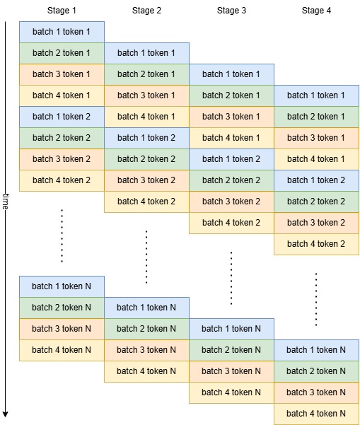
Pipeline Parallel (PP)
Shard on the number of layers. Each device will only compute a few layers of the model. At each time step, the device will receive the input data from previous pipeline stage (device), compute the layers, and then send the result to the next stage. However, PP requires the stages get balanced amount of work, otherwise all devices have to wait on the slowest stage and introduce huge overhead.
For LLMs, the majority of the workload are decoder layers, where input and output shapes are both \((B, S, H)\). For token generation, \(S = 1\) so that we that the send/recv communication is typically small. Also, token generation is auto-regressive, as illustrated below:
The overhead for pipelines are
- The idle time at the beginning and the end. For token generation, since the number of generated tokens are typically very large. This overhead is really small.
- Any load imbalance among stages where all other stages are idle.
- Send/recv communications in between stage. However, note that send buffer (input) and recv buffer (output) are different, so we can hide this overhead if send and recv are async.
- The number of batches have to be greater or equal to the number of stages.
PP scaling characteristics - HBM usage: each device takes \(1/\text{PP}\) model weights and \(1/\text{PP}\) KV cache. - Throughput: linearly scales. However, with more PP stages, we need larger batch size, and hence large KV cache. Also, keeping a balanced workload will be harder for too many PP stages. - Latency: does not help.
- CC overhead: send/recv.
Sequence Pipeline Parallel (SPP)
For prefill, similar to SP, partition the input tokens into chunks and do pipeline parallel on the chunks. Compared to token generation, typically the idling time at the beginning and the end will be larger. Since the number of chunks can be partitioned is typically way smaller than the number of generated tokens.
Mixing Parallelism
In general, we can mix shard on inputs (DP), shard on weights (TP), and shard on layers (PP), such that \(TP\times DP\times PP\) equals the number of devices.
Let \(\text{HBM}\) be the total HBM pressure if we run it on a single device, then the minimal per-device HBM pressure (assume no dominated replication) will be \(\text{HBM} / TP / PP\).
Let \(T\) be the latency for computing one prompt on a single device, then the minimal per prompt latency (assume 0 overhead in parallelism) will be \(T / TP\).
Case Study: llama3-70b
llama3-70b's parameters are
{
  "hidden_size": 8192,
  "intermediate_size": 28672,
  "num_attention_heads": 64,
  "num_key_value_heads": 8,
  "head_dim": 128,
  "num_hidden_layers": 80,
  "torch_dtype": "bfloat16",
  "vocab_size": 128256
}
So the HBM usage is
from math import ceil

# model configs
byte_size = 2 # bfloat16 is 2 bytes
n_layers = 80
H = 8192
I = 28672
n_q = 64
n_kv = 8
d_head = 128
vocab = 128256

for TP in (1, 4, 8, 64):
    n_kv_heads = ceil(n_kv / TP)
    n_heads = ceil(n_q / TP) + n_kv_heads * 2

    weights_total = sum([
        vocab / TP * H * byte_size, # embedding_w
        (n_heads * d_head) * H * n_layers * byte_size, # QKV_w
        (n_heads * d_head) * H * n_layers * byte_size, # out_w
        3 * (H / TP * I) * n_layers * byte_size, # gate_w + up_w + down_w
        2 * H * n_layers * byte_size, # norm_w, 2 RMS norm per layer
        vocab * H / TP * byte_size# lm_head_w
    ]) / 1024 / 1024 / 1024

    kv_cache_per_tok = 2 * n_kv_heads * d_head * n_layers * byte_size / 1024 / 1024
    print(f"TP={TP}")
    print(f"Total weights: {weights_total: .2f}Gb")
    print(f"KV Cache per token: {kv_cache_per_tok : .4f}Mb")

# TP=1
# Total weights:  133.92Gb
# KV Cache per token:  0.3125Mb
# TP=4
# Total weights:  33.48Gb
# KV Cache per token:  0.0781Mb
# TP=8
# Total weights:  16.74Gb
# KV Cache per token:  0.0391Mb
# TP=64
# Total weights:  2.64Gb
# KV Cache per token:  0.0391Mb
Consider the following accelerator server setup on AWS EC2: p5.48xlarge (NVIDIA DGX H100 System) vs trn2.48xlarge (Trainium2 server). They offer similar level of FLOPS, but the device configurations are different:
p5.48xlarge | trn2.48xlarge | |
|---|---|---|
| Number of devices | 8x H100 | 64x trn2 core |
| HBM size | 80Gb | 24Gb |
| HBM-cache bandwidth | 3350Gbs | 720 Gbs |
| bf16 FLOPS | * 989T | 153.6T |
| arithmetic intensity (FLOP/byte) | 295.2 | 213.3 |
* For sparse compute, H100 can deliver 1900T FLOPS
p5.48xlarge | trn2.48xlarge | |||
|---|---|---|---|---|
| Config | TP8 | TP4 DP2 | TP64 | TP8 DP8 |
| weight size (Gb) | 16.74 | 33.48 | 2.64Gb | 16.74 |
| per token KV cache (Mb) | 0.039 | 0.078 | 0.039 | 0.039 |
| max cached tokens (k) | 1600 | 590 | 545 | 185 |
| max B for 2.5k context | 640 | 236 | 218 | 74 |
From the table, we can observe a main limitation of trn2.48xl setup. For TP64, without considering the much larger communication overhead, we have to replicate 8 times for the weights loading and computations for K, V head projection, while for TP8 DP8, the maximum batch size is too small to get close to compute bound.