LLM Basics

The note will focus on transformer-based large language models, their inference pass, and some implementation basics. The note mainly use LLaMA series Dubey et al. [2024]¹ as a model example, and hunggingface/transformers as a reference for LLM framework implementation.

Additional resources: - huggingface/nlp-course - GPT from scratch by Jay Mody

Pipeline Components

As a high-level view, a LLM inference pipeline consists of

• tokenizer: input natural language text stream, output tokens.
• embedding: maps the tokens into a numerical format so that the model can consume.
• model: the actual LLM model, which takes the embedding and outputs according to the model tasks.
  • A typical transformer model has a encoder (plus positional encoding) to encode the input into feature vectors, a decoder that takes the features and other inputs to generate outputs.
  • Primarily if we consider the text generation task, we only need a decoder.
• postprocessing: Take the outputs from the model (often logits of embeddings), and format them back to text.

Tokenizers

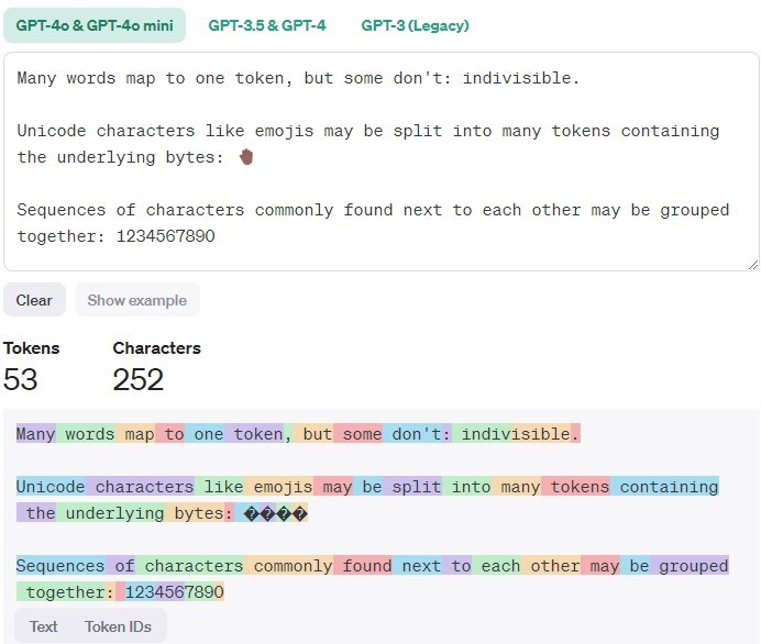
In general, tokenizer split the characters into sequences of tokens. In also handles irregular or illegal input, do normalization (striping whitespace, remove accent chars, lowercasing, etc.).

A simple view is to consider the token as one word, but not always true. Typically, the tokenizer only uses CPU, but not always true for some modern models.

from tokenizer import Tokenizer
tokenizer = Tokenizer.from_file("tokenizer.json")
output = tokenizer.encode("Hello, y'all! How are you 😁 ?")
print(output.tokens)
# ["Hello", ",", "y", "'", "all", "!", "How", "are", "you", "[UNK]", "?"]
print(output.ids)
# [27253, 16, 93, 11, 5097, 5, 7961, 5112, 6218, 0, 35]

Note that the tokenizer is often associated with the specific model.

Embedding

The tokenizer generate a sequence of tokens (or token IDs), but the model cannot directly consume them as input. Using an embedding, which serve as a fixed size dictionary of all tokens.

In general, we will also add a positional encoding to add an extra understanding of where the input is within the sentence.

# embedding is a lookup table of size (n_vocab, dim)
embeddings = Embedding(
    num_embedding=n_vocab, # number of vocab
    embedding_dim=embedding_dim # a configurable dim for embedding
)
# pos_encoder is a Encoding of size (max_seq_len, dim)
pos_encoder = PositionalEncoding(
    seq_len=max_seq_len, # configurable maximum sequence length
    dim=embedding_dim
)
# token_ids: Array[Int], shape (seq_len, )
# x: Array[Float], shape (seq_len, dim)
x = embeddings[token_ids] + pos_encoder[range(len(token_ids))]

Decoder-only Transformers

We focus on the auto-regressive models, or the decoder-only transformer models.

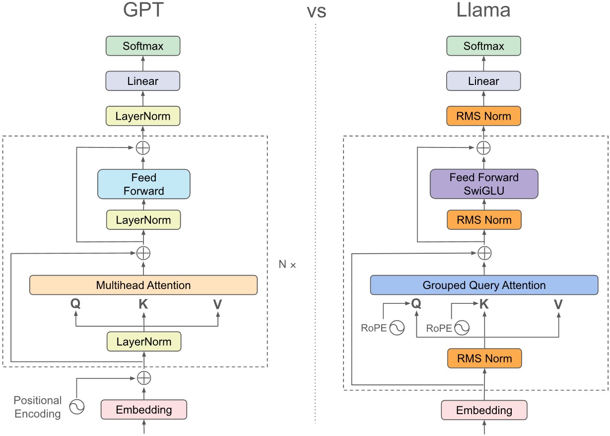
The embedding is passed through many Transformer blocks, and finally outputs the logits of the vocabulary to generate the next most likely word.

Attention Module

Consider an intuitive example: we have a set of word keys \(k_1, k_2, ..., k_n\) and each word \(k_i\) is associated with some feature vector \(v_i\), now we have a new word \(q\) to query, and we'd like to compute the value vector \(v_q = \sum_{i=1}^n a_i v_i\) with some attention score \(a_i\), and such \(a_i\) represents how similar/relevant is the query to the \(i\)th word.

Therefore, let \(K\: (n_k\times d_k)\) be the stacked matrix of keys, \(V\: (n_k\times d_v)\) be the stacked matrix of value vectors, and \(Q: (n_q\times d_v)\) be the stack matrix of queries. We can derive the attention to be

(See an intuitive explanation from Jay Mody, and detailed derivation in Attention is all You Need[Vaswani 2017]²)

Self-attention

An interesting discovery is that \(k\) and \(v\) can come from the same source, and we gets self attention, i.e. input sequence attend to itself. which means attention(q=x, k=x, v=x), which is just the similarity of all the words \(A = \text{softmax}(XX^T/\sqrt{d_k}) X\) to each other in the sentence, and no trainable parameters to embed the global context.

Therefore, we can introduce projections for the input \(Q = W_Q X, K = W_K X, V=W_VX\) and bring it back to original dimension by \(Y = W_{proj} A\), all the weight matrices are now trainable. In practice, we can stack \(W_Q, W_K, W_V\) into one matrix to combine the multiplication for a better parallelism.

Multi-head (MHA)

To have a truly "large" language model, we want the projections to have more parameters. However, \(QK^T\) part of the attention takes

Multi-head is introduced to reduce computation, in which we split the \(d_K, d_V\) into \(h\) "heads", i.e. smaller, separated features vectors. We compute attention on each and stack them back, so that the computation is

In implementation, MHA with \(N\) heads looks like \(A_i = \text{softmax}(\frac{(W_Q^iQ)\cdot (W_K^i K)^T}{\sqrt{d_k}}) W_V^iV\), \(MHA = W_O\cdot \text{concat}(A_1, A_2, ..., A_{N})\), where \(W_O\) is the weights for output projection.

Group Query (GQA) and Multi-query (MQA)

Instead of using multi-head on all of \(Q,K,V\), MQA only use the full multi heads on \(Q\).

Note that we only have one weight for \(W_K\) and \(W_V\), instead of \(n\) weights.

GQA uses the similar idea, instead of all \(N\) heads of query share the same projected \(K, V\), we have \(N/d\) heads for \(K,V\) and every \(d\) Q-heads will share one KV head.

Causal Masking

For a text generation model, all words should only see words before it. Otherwise, it will be biased towards the known answer.

One natural way is to mask out the relevance in the context. Which means \(0\) for all the keys after the current key. However, we need to pass a softmax and have \(0\) in the output. We can do this by adding a negative-infinity matrix \(M\) to \(QK^T\).

KV Caching for Casual Inference

For text generation tasks with a transformer model, the inference is done as

prompt_tokens = tokenizer.encode(input_text)

for _ in range(n_next_tokens):
    new_token = model(prompt_tokens)
    prompt_tokens.append(new_token)

output_tokens = tokenizer.decode(prompt_tokens)

Because we always want to generate new tokens based on all previous context. However, in each iteration we only have 1 new token, we are always recomputing the prompt tokens. Considering the computation in attention module, the overhead is exponential to the max_sequence_len.

However, casual inference masks out tokens after the current token. For each queried token, its attention \(A, Q, K, V\) are only relevant to previous tokens. Therefore, for each iteration - We only need to query the newly generated input. - We reuse all previous \(K,V\), concat with the new \(k, v\) w.r.t input \(x\).

The inference becomes

prompt_tokens = tokenizer.encode(input_text)

# context encoding phase
# K_cache, V_cache shape (len(prompt_tokens), ...)
new_token, K_cache, V_cache = model(
    prompt_tokens, K_cache=[], V_cache=[])
propmpt_tokens.append(new_token)

# token generation phase
for _ in range(n_next_tokens):
    # new_K_cache, new_V_cache, shape (1, ...)
    new_token, new_K_cache, new_V_cache = model(
        new_token, K_cache=K_cache, V_cache=V_cache)
    K_cache.append(new_K_cache)
    V_cache.append(new_V_cache)
    prompt_tokens.append(new_token)

output_tokens = tokenizer.decode(prompt_tokens)

Putting all Together

# forward part of Attention module from llama3
# https://github.com/meta-llama/llama3/blob/main/llama/model.py
def forward(
    self,
    x: torch.Tensor,
    start_pos: int,
    freqs_cis: torch.Tensor,
    mask: Optional[torch.Tensor],
):
    bsz, seqlen, _ = x.shape

    # projections
    xq, xk, xv = self.wq(x), self.wk(x), self.wv(x)

    xq = xq.view(bsz, seqlen, self.n_local_heads, self.head_dim)
    xk = xk.view(bsz, seqlen, self.n_local_kv_heads, self.head_dim)
    xv = xv.view(bsz, seqlen, self.n_local_kv_heads, self.head_dim)

    # llama3's rotary positional encoding
    # refer to the original paper for detail
    xq, xk = apply_rotary_emb(xq, xk, freqs_cis=freqs_cis)

    # KV caching
    self.cache_k = self.cache_k.to(xq)
    self.cache_v = self.cache_v.to(xq)

    self.cache_k[:bsz, start_pos : start_pos + seqlen] = xk
    self.cache_v[:bsz, start_pos : start_pos + seqlen] = xv

    keys = self.cache_k[:bsz, : start_pos + seqlen]
    values = self.cache_v[:bsz, : start_pos + seqlen]

    # Multi-head

    # repeat k/v heads if n_kv_heads < n_heads
    keys = repeat_kv(
        keys, self.n_rep
    )  # (bs, cache_len + seqlen, n_local_heads, head_dim)
    values = repeat_kv(
        values, self.n_rep
    )  # (bs, cache_len + seqlen, n_local_heads, head_dim)

    xq = xq.transpose(1, 2)  # (bs, n_local_heads, seqlen, head_dim)
    keys = keys.transpose(1, 2)  
    # (bs, n_local_heads, cache_len + seqlen, head_dim)
    values = values.transpose(1, 2)  
    # (bs, n_local_heads, cache_len + seqlen, head_dim)

    # self-attention
    scores = torch.matmul(xq, keys.transpose(2, 3)) / math.sqrt(self.head_dim)
    if mask is not None:
        scores = scores + mask  # (bs, n_local_heads, seqlen, cache_len + seqlen)
    scores = F.softmax(scores.float(), dim=-1).type_as(xq)
    output = torch.matmul(scores, values)  # (bs, n_local_heads, seqlen, head_dim)
    output = output.transpose(1, 2).contiguous().view(bsz, seqlen, -1)

    # projection back
    return self.wo(output)

Feed forward Network

Simple fully connected linear layers to expand and contract the embedding dimension, so that we have more trainable weights for the context. For LLaMA3 the design is a bit different to have more efficiency.

# https://github.com/meta-llama/llama3/blob/main/llama/model.py
class FeedForward(nn.Module):
    def __init__(
        self,
        dim: int,
        hidden_dim: int,
        multiple_of: int,
        ffn_dim_multiplier: Optional[float],
    ):
        super().__init__()
        hidden_dim = int(2 * hidden_dim / 3)
        # custom dim factor multiplier
        if ffn_dim_multiplier is not None:
            hidden_dim = int(ffn_dim_multiplier * hidden_dim)
        hidden_dim = multiple_of * ((hidden_dim + multiple_of - 1) // multiple_of)

        self.w1 = ColumnParallelLinear(
            dim, hidden_dim, bias=False, gather_output=False, init_method=lambda x: x
        )
        self.w2 = RowParallelLinear(
            hidden_dim, dim, bias=False, input_is_parallel=True, init_method=lambda x: x
        )
        self.w3 = ColumnParallelLinear(
            dim, hidden_dim, bias=False, gather_output=False, init_method=lambda x: x
        )

    def forward(self, x):
        return self.w2(F.silu(self.w1(x)) * self.w3(x))

Inference Acceleration and Performance Evaluation

All About Transformer Inference - How to Scale Your Model with TPU

During inference, we are optimizing for time to first token (TTFT) and tokens per second (TPS). Without changing the actual computations, we want fully use the hardware, i.e. better model FLOPS utilization (MFU) and model bandwidth utilization (MBU) at the same time.

On a typical hardware (CPU/GPU/TPU), we have a memory hierarchy, where data needs to be loaded from the large-sized memory (often HBM) to the much smaller cache/register (SBUF) for computation. The data movement can be seen as executed by DMA engines, and can be overlapped with computations. Therefore, the theoretical performance is max(data_movement_time, computation_time). This is called the roofline model.

Q, K, V projection

Q, K, V projection \([Q_p, K_p, V_p] = [W_Q\cdot Q, W_K\cdot K, W_V\cdot V]\) where

• \(Q,K,V: (1, H, S)\), \(S\) is sequence length, \(H\) is hidden dimension size
• \(W_Q, W_K, W_V: (N_{heads}, I, H)\), \(N_{heads}\) is number of heads, \(I\) is intermediate dimension size.
• \(Q_p, K_p, V_p: (N_{heads}, I, S)\) are the projected multi-head values

So total flop is \(3N_{heads} \times 2IHS = 6N_{heads}IHS\), data movement is \(N_{bytes}\times(HS+N_{heads}IH+BF)\), where \(N_{bytes}\) depends on dtype.

Flash Attention

Flash Attention[Dao et al. 2022]³ is a widely-used method for optimizing attention computations. We will only talk about forward pass here.

In the attention computation, we are doing two large matmul, one division (which can be pre-applied) and one softmax. In which we have to write the result back to HBM for each operation. A natural way to improve is to use the fused operations, i.e. re-order/design the computations so that we do not write intermediate results back to HBM. Fusing matmuls is easy: assuming SBUF can fit at least 3 hidden vectors, we partition \(QKV\) by the sequence dim. If we ignore the softmax part, we have two matmuls and fuse the computation of \(S_P\) tokens: \([(S_P , I) \times (I, S_P)]\times (S_P, I) = (S_P, S_P)\times (S_P, I) = (S_P, I)\)

Now, consider the softmax, for numerical stability we have to use standard normalized softmax

If we partition \(\mathbf{x}\) into \([\mathbf{x}_1, \mathbf{x}_2]\), then \(m_1 = \max(\mathbf{x}_1), m_2 = \max(\mathbf{x}_2), m = \max(m_1, m_2)\), then

Also observe that

Which means that for each partition, we only need to keep \(\exp(\mathbf x_1 - m_1), m_1\) and the denominator \(l_1 := \exp(\mathbf x_1 - m_1)\). Also, since \(m_1, l_1\) are scalar multiplication, we would postbone the reduction after the matmuls.