Multivalued Functions

Square Root Function

Consider the simplest example, for \(z = w^2\), we can write its inverse as \(w = z^{1/2}\), we know that its \(z^{1/2}\) have values as

\[z^{1/2} \equiv \sqrt r e^{i\frac{\theta + 2\pi n }{2}}, n = 0, 1, 2, ...\]

Which takes to be 2 distinct values \(\pm \sqrt r e^{i\theta/2}\).

Therefore, if we define some function f as one root of the square root function, say \(f(re^{i\theta}) = \sqrt{r} e^{i\theta/2}\).
Consider a path traverse through the circle of radius \(r\) around \(0\),

\[c:[0, 2\pi)\rightarrow \mathbb C, c(t) = re^{it}, c(0) = c(2\pi) = r\]

Then, consider any \(t\in(0, 2\pi)\), \(f(c(t))\) is continuous. However, when \(f\) goes along the path and approaches \(2\pi\), we have

\[\lim_{t\rightarrow 2\pi} f(c(t)) = \sqrt re^{i\pi} = -\sqrt r\neq \sqrt r = f(c(0))\]

\(f\) does not return to its original value.

If we look at another example (fig.2), consider a path traverse through the circle around \(1.1+1.1i\). \(f\) goes back to the original value.

Source code

import matplotlib.pyplot as plt
import numpy as np

def angle(z):
    # since np.angle uses y-axis as branch cut, 
    # we need to change it to x-axis
    theta_pos = np.angle(z) * (z.imag > 0)
    theta_neg = (np.angle(z) + 2 * np.pi) * (z.imag < 0)
    return theta_pos + theta_neg
def sqrt(z):
    # define our sqrt function with branch cut y=0
    return np.abs(z)**.5 * np.exp(1j * (angle(z)/2))

t = np.arange(0, 2 * np.pi, np.pi/100)
c = np.array([
    1.2 * np.exp(1j * t[:, np.newaxis]),
    1.1 + np.exp(1j * t[:, np.newaxis]),
    1.1j + np.exp(1j * t[:, np.newaxis]),
    1.1 + 1.1j + np.exp(1j * t[:, np.newaxis]),
])
c_func = [
    '$c(t) = 1.2e^{it}$',
    '$c(t) = 1.1 + e^{it}$',
    '$c(t) = 1.1i + e^{it}$',
    '$c(t) = 1.1 + 1.1i + e^{it}$'
]
fc = sqrt(c)
fig = plt.figure(figsize=(16, 4))
fig.suptitle(r"f defined as $\sqrt{r} e^{i\theta/2}$", y=0)
for i in range(c.shape[0]):
    plt.subplot(1, 4, 1+i)
    plt.xlim(-3, 3); plt.ylim(-3, 3)
    plt.gca().set_aspect('equal')
    plt.axhline(c="grey", ls="--"); plt.axvline(c="grey", ls="--"); 
    plt.scatter(c[i].real, c[i].imag, s=.5); plt.scatter(fc[i].real, fc[i].imag, s=.5)
    plt.title(f"fig{i}. " + c_func[i])
plt.savefig("../assets/multi_val_func_01.jpg")

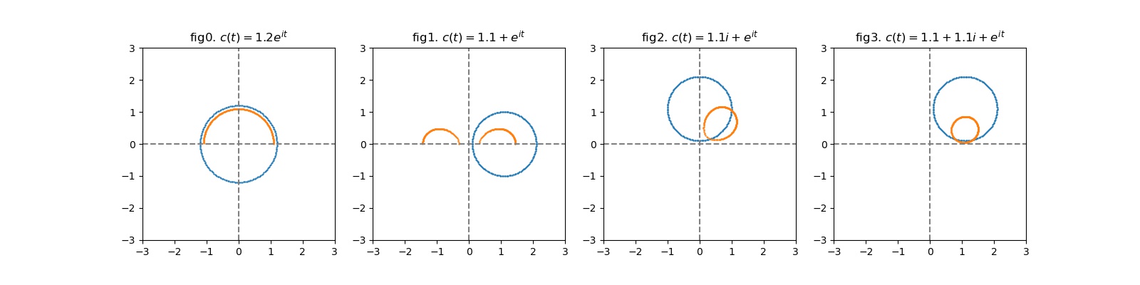
Note that for the curve traversed by \(c(t)= 1.1+e^{it}\), there exists some other definition of \(f\) as square root function such that the image of \(f\) can be closed.

Branch

Therefore, we define a branch point for a multivalued function \(f\) as
- (intuitively) \(f\) is discontinuous upon traversing a small circuit around the point - (more formally) \(z_0\) is a branch point if there is no domain \(D\) on which a continuous single value functions that is defined which contains \(B_\delta(z_0) - \{z_0\}\) for any \(\delta > 0\).

For example, the square root function have branch points \(0, \infty\).

A branch of a multivalued function is a single valued continuous function defined on a restricted region.

For functions with a single branch point, \(z_0\), a branch cut is a curve \(p:[0,\infty)\rightarrow \mathbb C\), s.t. \(p(0) = z_0, p(\infty) = \infty\), so that a branch can be defined on \(\mathbb C - p([0,\infty))\)

Logarithm Function

Consider the inverse of exponential function \(w = f(z)\) s.t. \(e^w = z\).

\[\begin{align*} e^w &= z\\ e^{u+iv} &= re^{i\theta} &u,v\in\mathbb R, r > 0, \theta\in [0, 2\pi)\\ e^ue^{iv} &= re^{i\theta}\\ e^u = r&\Rightarrow u = \log(r)\\ v &= \theta + 2\pi n\\ \Rightarrow w &= log(r) + i(\theta + 2\pi n) &n\in\mathbb Z \end{align*}\]

This is multivalued, and in fact, it has infinite distinct values for each \(n\) chosen.

Conveniently, we take \(n = 0\) and defines the principal branch of \(\log\) on the domain \(D = \{re^{i\theta} :r > 0, \theta \in [0, 2\pi)\}\) as

\[\log: D\rightarrow \mathbb C, \log(re^{i\theta}):= \log r + i\theta\]

Power Function

Note that the power function can be defined through

\[z^a = (e^{\log z})^a = e^{a\log z}\]

Consider \(a = n\in\mathbb Z\),

\[\begin{align*} \exp({n\log(re^{i\theta}))} &\equiv \exp(n(\log r + i\theta + i2\pi k)) \\ &= e^{n\log r} \cdot e^{in\theta} \cdot e^{i2\pi (nk)} \\ &= r^n\cdot e^{in\theta}\cdot 1 \\ &= r^n (e^{i\theta})^n \\ &= (re^{i\theta})^n \end{align*}\]

it is uniquely defined

However, for \(a = n^{-1}\),

\[\begin{align*} \exp({n^{-1}\log(re^{i\theta}))} &\equiv \exp(n^{-1}(\log r + i\theta + i2\pi k)) \\ &= e^{\frac{\log r}{n}} \cdot e^{i\frac{\theta}n} \cdot e^{i \frac{2\pi k}{n}} \\ &= r^{1/n}\cdot e^{i\frac{\theta}n}\cdot e^{i \frac{2\pi k}{n}} \\ &= (re^{i\theta})^{1/n}e^{i \frac{2\pi k}{n}} \end{align*}\]

it has \(n\) different values

Finally, for \(a = i\),

\[\begin{align*} \exp(i\log z) &\equiv \exp(i(\log r + i\theta + i2\pi k)) \\ &=e^{i\log r} e^{-\theta}e^{-2\pi k} \end{align*}\]

it has infinitely many values

Example

For \(a\in\mathbb R\). Show that the set of all values of \(\log(z^a)\) is not necessarily the same as \(a\log(z)\).

Consider \(z = re^{i\theta}\) for \(r > 0, \theta \in [0, 2\pi)\).

\[\begin{align*} \log(z^a) &= \log(r^ae^{ia\theta}) = a\log(r) + i(a\theta + 2\pi k)\\ a\log(z) &= a\log(re^{i\theta}) = a\log(r) + ia(\theta + 2\pi k) \end{align*}\]

Note that \(\{(a\theta + 2\pi ak):k\in\mathbb Z\} \neq \{a\theta + 2\pi k):k\in\mathbb Z\}\)