Image Pyramids

Image Downsampling

Initial thought

To resize of image to \(\frac{1}{n}\), resample the image by picking pixel per \(n\) pixels

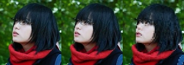
Problem: Aliasing

Occurs when sampling rate is not high enough to capture the amount of detail in the image.

Below is an extremum, which we lost half of the important information

Nyquist rate

To avoid such aliasing issue, one should sample at least \(2\times \max{f}\), i.e. at least twice the highest frequency.

With twice the frequency, we can make sure the information is caught, while in other cases, it might not be true

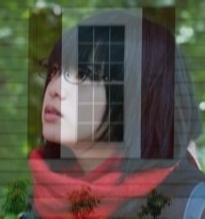
Gaussian pre-filtering

When downsampling, the original image has too high frequencies, results in information loss. The high frequencies are caused by shape edges, hence we can smooth the image to filter out high frequencies, with a low-pass filter

Gaussian Pyramids

A sequence of images created with Gaussian blurring and downsampling is called a Gaussian pyramid or mip map

Image Up-Sampling

Interpolation

Since an image is a discrete point-sampling of a continuous function, i.e. \(F(x,y) = quantize\{f(x/d, y/d)\}\). If we could somehow reconstruct the original continuous function, we can generate the image with any resolution and scale.

However, we are unable to obtain such \(f\), but we can guess an approximation

Nearest neighbor

\[f(x) = F(\arg\min\{d(x - x_i)\})\]

Linear interpolation

Given \(x \in [x_i, x_{i+1}], G(x) = \frac{x_{i+1}-x}{x_{i+1}-x_i}F(x_i) + \frac{x-x_{i+1}}{x_{i+1}-x_i}F(x_{i+1})\)

Via Convolution 1D

To upsampling a line \(F= p_1, p_2, ..., p_n\),
insert \(n*0\)s between \(p_i, p_{i+1}\), make into \(G = p_i. 0, 0, ..., 0, p_{i+1}\)
Take convolution filter \(h = [0, 1/d, 2/d, ..., d/d, (d-1)/d, ... 0]\)
\(h*G\) is desired

Similar idea goes to 2D

Bilinear interpolation

Given \(Q_{00}=(x_0,y_0), Q_{01}=(x_0, y_1), Q_{10}=(x_1,y_0), Q_{11}=(x_1,y_1)\).
Interpolate along \(x\)-axis

\[F(x,y_0)\approx \frac{x_1 - x}{x_1 - x_0}F(Q_{00}) +\frac{x - x_0}{x_1 - x_0}F(Q_{10})\]

\[F(x,y_1)\approx \frac{x_1 - x}{x_1 - x_0}F(Q_{01}) +\frac{x - x_0}{x_1 - x_0}F(Q_{11})\]

Then, interpolate along \(y\)-axis

\[F(x,y) \approx \frac{y_1 - x}{y_1 - y_0}F(x,y_0) +\frac{y - y_0}{y_1 - y_0}F(x,y_1)\]

\[\begin{align*} F(x,y)= &\frac{(x_1-x)(y_1-y)}{(x_1-x_0)(y_1-y_0)}F(Q_{00})\\ + &\frac{(x-x_0)(y_1-y)}{(x_1-x_0)(y_1-y_0)}F(Q_{10})\\ + &\frac{(x_1-x)(y-y_0)}{(x_1-x_0)(y_1-y_0)}F(Q_{01})\\ +&\frac{(x-x_0)(y-y_0)}{(x_1-x_0)(y_1-y_0)}F(Q_{11}) \end{align*}\]

Therefore, suppose \(\|x_1-x_0\| = \|y_1-y_0\| = 1\), i.e. the 4 points form a unit square, and let \(x-x_0 = d_x, y-y_0 = d_y\).

\[F(x,y)=(1-d_x)(1-d_y)F(Q_{00})+d_x(1-d_y)F(Q_{10}) + (1-d_x)d_yF(Q_{01}) + d_xd_yF(Q_{11})\]

Which can be represented by the dot product of \(\vec v^T \cdot \vec v\) where \(v\) is the vector filter in 1-D case.

Source code

import cv2
import numpy as np
import plotly.graph_objects as go

img = cv2.imread("../assets/yurina.jpg")

H, W, C = img.shape
output = np.zeros((H, W * 3, C), dtype=np.uint8)
output[:, :W, :] = img
output[:, W:2*W, :] = cv2.resize(img[::2,::2,:], (W, H), interpolation=cv2.INTER_NEAREST)
output[:, 2*W:, :] = cv2.resize(img[::4,::4,:], (W, H), interpolation=cv2.INTER_NEAREST)
cv2.imwrite("../assets/image_downsample.jpg", output)


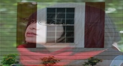
img2 = cv2.imread("../assets/window.jpg")
img2 = cv2.resize(img2, (W, H))
output = np.empty((H, W*2, 3), dtype=np.uint8)
for i in range(img.shape[1]):
    output[:, 2*i] = img2[:, i]
    output[:, 2*i+1] = img[:, i]
cv2.imwrite("../assets/image_downsample_2.jpg", output)



x = np.arange(0, 40, 0.2)
x2 = np.arange(0, 40, 3)
fig = go.Figure(data=[
    go.Scatter(x=x, y=np.cos(x), name="sample rate=0.2"),
    go.Scatter(x=x2,y=np.cos(x2), name="sample rate=3")
])
with open("../assets/nyquist_cos.json", "w") as f:
    f.write(fig.to_json())

img3 = cv2.GaussianBlur(output, (3, 3), 3)[:, ::2]
cv2.imwrite("../assets/image_downsample_3.jpg", img3)