Variational Autoencoders
Dimension Reduction and Autoencoder Basics
Autoencoders
As a recap, an encoder-decoder is a fair of function (often non-linear functions implmented as neural networks).
- Encoder \(g: D\rightarrow F\)
- Decoder \(f: F\rightarrow D\)
where \(D\) is the input space, \(F\) is the feature vector, where \(\dim(F)\ll \dim(D)\).
The goal of an atuoencoder is that for any input
Therefore, we could compress input data \(x\) into a lower dimension features, for storage, comparisons, visualizations, etc.
Proximity Issue
Note that \(f,g\) are non-linear, and decoder can not an inverse function of \(f\neq g^{-1}\). Thus, small change in the input space does not corresponds to small change in the feature space. In fact, \(f\) and \(g\) can acts as some hashing functions that prevents proximity.
In addition, if the data space has discontinuities, for example, several clusters with remote means and small variance. Then, if we sample from the "vacuum" in the input space, then the feature can be totally random.
Variational Autoencoders
VAEs solve proximity issue by introducing uncertainty. By adding noise, VAEs force the encoder to output more uniformly continuous results. The encoder outputs a distribution \(q_\theta(z|x)\) instead of a deterministic feature vector. Normally, we will use Gaussian distribution for \(q\), so that encoder outputs \((\mu, \sigma) = f(x)\), in practice \(\Sigma\) is the diagonal matrix.
The idea of VAE comes from variational inference. Let the feature vector be the laten variable, and input data be the observations, the autoencoder aims to recover the posterior \(p(z|x)\) from likelihood and prior. And we use \(q_\theta\) to approximate such \(p\) due to computational limits. For optimization / training VAEs, we use ELBO as its loss. Thus, we have
- Encoder \(q_{\phi_i}(z|x_i) = \mathcal N(\mu_i, \sigma_i^2)\) where we store the mean \(\mu_i\) and log std \(\sigma_i\) for each input.
- Decoder \(f(z_i) = \tilde \theta\), typically a neural network that output parameters for a class of distribution.
Pipeline
For each given input \(x_i\), we have the forward path as
- The encoder NN \(g\) output \(\phi_i = g(x_i)\).
- Sample latent vector \(z_i \sim q_{\phi_i}(z|x_i)\).
- The decoder NN \(f\) output \(\theta = f(z_i)\).
- Sample decoded sample \(\hat x_i = p_{\theta}(x|z)\)
Consider the backward path, we have two ELBOs for \(p_\theta\) and \(q_\phi\) be the losses, note that ELBO loss requires the reparameterization tricks, similar to VI.
Amortized VAE
Instead of doing VI from scratch for each \(x_i\), we learn a function that can look at the dataset all together. Therefore, instead of learning separate parameters \(\phi_i\) for each input, we learn a single global distribution \(\phi\) that specifies the parameters of the recognition model, and \(\phi\) is the parameter sets we want to store.
The basic for AVAE pipeline is very similar to VAE, except that we now have a high-dimensional model. Thus, we sample from
Implementation Example: MNIST
Using the classical MNIST example
- Input data: \(28 * 28\) pixels of value \([0,1]\), representing grayscale.
- Likelihood function \(p_\theta(x|z) = \text{Bernoulli}(\theta)\)
- Approximate posterior \(q_{\phi_i}(z|x_i) = \mathcal N(\mu_i, \sigma_i)\)
- Loss be the ELBO loss + Reconstruction loss
 class VAE(nn.Module):
     def __init__(self, x_dim, h_dim1, h_dim2, z_dim):
         super(VAE, self).__init__()

         # encoder part
         self.fc1 = nn.Linear(x_dim, h_dim1)
         self.fc2 = nn.Linear(h_dim1, h_dim2)
         self.fc31 = nn.Linear(h_dim2, z_dim)
         self.fc32 = nn.Linear(h_dim2, z_dim)
         # decoder part
         self.fc4 = nn.Linear(z_dim, h_dim2)
         self.fc5 = nn.Linear(h_dim2, h_dim1)
         self.fc6 = nn.Linear(h_dim1, x_dim)

     def encoder(self, x):
         h = F.relu(self.fc1(x))
         h = F.relu(self.fc2(h))
         return self.fc31(h), self.fc32(h) # mu, log_var

     def sampling(self, mu, log_var):
         std = torch.exp(0.5*log_var)
         eps = torch.randn_like(std)
         return eps.mul(std).add_(mu) # return z sample

     def decoder(self, z):
         h = F.relu(self.fc4(z))
         h = F.relu(self.fc5(h))
         return torch.sigmoid(self.fc6(h))

     def forward(self, x):
         mu, log_var = self.encoder(x.view(-1, 784))
         z = self.sampling(mu, log_var)
         return self.decoder(z), mu, log_var

 def ELBO_loss(recon_x, x, mu, log_var):
     # ~ Bernoulli ELBO
     BCE = F.binary_cross_entropy(recon_x, x.view(-1, 784), reduction='sum')
     # Normal ELBO
     KLD = -0.5 * torch.sum(1 + log_var - mu.pow(2) - log_var.exp())
     return BCE + KLD

 def train(model, train_loader, optimizer):
     model.train()
     train_loss = 0
     for data, _ in train_loader:
         data = data.cuda()
         optimizer.zero_grad()
         recon_batch, mu, log_var = model(data)
         loss = ELBO_loss(recon_batch, data, mu, log_var)
         loss.backward()
         train_loss += loss.item()
         optimizer.step()
     return train_loss / len(train_loader.dataset)

 def test(model, test_loader):
     model.eval()
     test_loss= 0
     with torch.no_grad():
         for data, _ in test_loader:
             data = data.cuda()
             recon, mu, log_var = model(data)
             # sum up batch loss
             test_loss += ELBO_loss(recon, data, mu, log_var).item()
     return test_loss / len(test_loader.dataset)

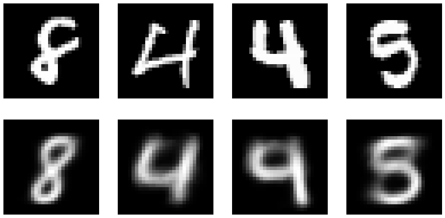
The reconstruction
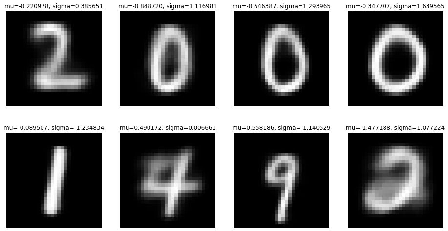
Random samples from the hidden vector code
Source code
import torch
import torch.nn as nn
import torch.nn.functional as F
from torchvision import datasets, transforms
import numpy as np
import matplotlib.pyplot as plt


# --8<-- [start:vae]
class VAE(nn.Module):
    def __init__(self, x_dim, h_dim1, h_dim2, z_dim):
        super(VAE, self).__init__()

        # encoder part
        self.fc1 = nn.Linear(x_dim, h_dim1)
        self.fc2 = nn.Linear(h_dim1, h_dim2)
        self.fc31 = nn.Linear(h_dim2, z_dim)
        self.fc32 = nn.Linear(h_dim2, z_dim)
        # decoder part
        self.fc4 = nn.Linear(z_dim, h_dim2)
        self.fc5 = nn.Linear(h_dim2, h_dim1)
        self.fc6 = nn.Linear(h_dim1, x_dim)

    def encoder(self, x):
        h = F.relu(self.fc1(x))
        h = F.relu(self.fc2(h))
        return self.fc31(h), self.fc32(h) # mu, log_var

    def sampling(self, mu, log_var):
        std = torch.exp(0.5*log_var)
        eps = torch.randn_like(std)
        return eps.mul(std).add_(mu) # return z sample

    def decoder(self, z):
        h = F.relu(self.fc4(z))
        h = F.relu(self.fc5(h))
        return torch.sigmoid(self.fc6(h))

    def forward(self, x):
        mu, log_var = self.encoder(x.view(-1, 784))
        z = self.sampling(mu, log_var)
        return self.decoder(z), mu, log_var

def ELBO_loss(recon_x, x, mu, log_var):
    # ~ Bernoulli ELBO
    BCE = F.binary_cross_entropy(recon_x, x.view(-1, 784), reduction='sum')
    # Normal ELBO
    KLD = -0.5 * torch.sum(1 + log_var - mu.pow(2) - log_var.exp())
    return BCE + KLD

def train(model, train_loader, optimizer):
    model.train()
    train_loss = 0
    for data, _ in train_loader:
        data = data.cuda()
        optimizer.zero_grad()
        recon_batch, mu, log_var = model(data)
        loss = ELBO_loss(recon_batch, data, mu, log_var)
        loss.backward()
        train_loss += loss.item()
        optimizer.step()
    return train_loss / len(train_loader.dataset)

def test(model, test_loader):
    model.eval()
    test_loss= 0
    with torch.no_grad():
        for data, _ in test_loader:
            data = data.cuda()
            recon, mu, log_var = model(data)
            # sum up batch loss
            test_loss += ELBO_loss(recon, data, mu, log_var).item()
    return test_loss / len(test_loader.dataset)
# --8<-- [end:vae]

# MNIST Dataset
train_dataset = datasets.MNIST(root='./mnist_data/', train=True, transform=transforms.ToTensor(), download=True)
test_dataset = datasets.MNIST(root='./mnist_data/', train=False, transform=transforms.ToTensor(), download=False)
# Data Loader (Input Pipeline)
train_loader = torch.utils.data.DataLoader(dataset=train_dataset, batch_size=100, shuffle=True)
test_loader = torch.utils.data.DataLoader(dataset=test_dataset, batch_size=1000, shuffle=False)

# build model
vae = VAE(x_dim=784, h_dim1= 512, h_dim2=256, z_dim=2).cuda()
optimizer = torch.optim.Adam(vae.parameters())
nepoch = 40
train_loss = np.empty(nepoch)
test_loss = np.empty(nepoch)
from tqdm import tqdm
for epoch in tqdm(range(nepoch)):
    train_loss[epoch] = train(vae, train_loader, optimizer)
    test_loss[epoch] = test(vae, test_loader)

plt.figure(figsize=(6,4))
plt.title("Loss")
plt.plot(train_loss, label="train loss")
plt.plot(test_loss, label="test loss")
plt.savefig("../assets/vae_loss.png")


fig, axs = plt.subplots(2, 4, figsize=(16, 8))
from random import sample
with torch.no_grad():
  for i, idx in enumerate(sample(range(len(test_dataset)), 4)):
    input = test_dataset[idx][0]
    axs[0, i].imshow(input.view(28, 28).numpy(), cmap="gray")
    input = input.cuda()
    recon, mu, log_var  = vae(input)
    axs[1, i].imshow(recon.view(28, 28).detach().cpu().numpy(), cmap="gray")
    axs[1, i].set_axis_off(); axs[0, i].set_axis_off()
fig.savefig("../assets/vae_recons.png")


fig, axs = plt.subplots(2, 4, figsize=(16, 8.4))
with torch.no_grad():
  for i in range(8):
    z = torch.randn(2)
    axs[i%2, i//2].set_title(f"mu={z[0]:.6f}, sigma={z[1]:.6f}")
    z = z.cuda()
    sample = vae.decoder(z).cuda()
    axs[i%2, i//2].imshow(sample.view(28, 28).detach().cpu().numpy(), cmap="gray")
    axs[i%2, i//2].set_axis_off()
fig.savefig("../assets/vae_random.png")