Solve Non-linear equations

import numpy as np
import matplotlib.pyplot as plt
import pandas as pd

Example

solve \(f(x) = x^2 - 4\sin(x)= 0\), i.e. \(x^2 = 4\sin x\)

plt.figure(figsize=(4, 3))
x = np.arange(-4, 4, 0.01)
sq = x ** 2
sin = 4 * np.sin(x)
plt.plot(x, sq, label=r"$x^2$")
plt.plot(x, sin, label=r"$4\sin(x)$")
plt.legend()
plt.tight_layout()
plt.savefig("assets/non_linear_equations_1.jpg")

Noting that \(f(\pi/2) = (\pi/2)^2 - 4(1) < 0\) and \(f(2) = 2^2 - 4\sin(2)>0\), by IVT, \(\exists x\in(\pi/2, 2), f(x)=0\)

Solving non-linear Equations

For linear functions, it's easy to determine the number of roots, while for non-linear equations, this is harder.

Bisection Method

For continuous functions, using IVT, we can determine the minimum number of roots. Then, using this fact, we define a recursive algorithm

• find \(a, b\) s.t. \(f(a)f(b)\leq 0\)
• take \(m = (a+b)/2\), if \(f(a)f(m)\leq 0\), then the root \(x\in [a,m]\), otherwise \(f(b)f(m)\leq 0, x\in[m,b]\)

init a, b <= f(a)f(b) <= 0
while b - a > tolerance:
    m = (a + b) / 2
    if f(a)f(m) <= 0:
        a = m
    else:
        b = m

By nested interval theorem, we are guaranteed to find one solution.

Fixed Point Method

A point \(x^*\) is a fixed point of a function \(g\) if \(x^*=g(x^*)\)

Contraction Mapping Theorem

A function \(f:\mathbb R^n \rightarrow \mathbb R^n\) is a contraction if \(\exists \gamma < 1, \|f(x)-f(y)\| < \gamma \|x-y\|\), then \(\exists x^*, x^* = g(x^*)\), i.e. exists a fixed point.

proof (MAT337 Banach Contraction Principle

Therefore, fixed point method gives the algorithm

init x[0] from domain
x[1] = f(x[0])
i = 1
while abs( x[i+1] - x[i] ) >= tolerance:
    x[i+1] = f(x[i])
    i += 1

Rate of Convergence

Consider any iterative method for computing non-linear function solution. \(x^*\) being the exact solution (fixed point in FPM), then define \(e_k = x^* - x_k\) assuming \(x_k\rightarrow x^*\).
Suppose

Then the rate of convergence is defined as \(r\)

• \(r=1: c<1\) - linear convergence
• \(r>1\): super linear convergence
• \(r=2\): quadratic convergence

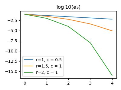
Example

Suppose we start with \(e_0 = 0.1\)

k = np.arange(5)
e = np.zeros((3, 5))
e[:, 0] = 0.1

for i in range(1, 5):
    e[0, i] = e[0, i-1] ** 1 * 1/2
    e[1, i] = e[1, i-1] ** 1.5
    e[2, i] = e[2, i-1] ** 2
plt.figure(figsize=(4, 3))
plt.plot(k, np.log10(e[0]), label="r=1, c = 0.5");
plt.plot(k, np.log10(e[1]), label="r=1.5, c = 1");
plt.plot(k, np.log10(e[2]), label="r=2, c = 1");
plt.legend()
plt.title(r"$\log10(e_k)$")
plt.tight_layout()
plt.savefig("assets/non_linear_equations_2.jpg")

Newton's Method

Replacing the function \(f(x)\) by its tangent line at the current point of approximation \(x^{(k)}\), assuming the function is differentiable at \(x^{(k)}\), i.e.

Then approximate the root of \(f(x)=0\), i.e. the point where the graph of \(f(x)\) hits the \(x\)-axis, by the point where the graph of the tangent hits the \(x\)-axis. We are looking for the point \(x\) s.t. \(y = 0\). This will be the new approximation \(x^{(k+1)}\) to the root of \(f\). Thus

Algorithm

init x[0]
for k in range(n):
    x[k] = x[k-1] - f(x[k-1]) / df(x[k-1])
    if abs(f(x[k])) < tolarence:
        return x[k]      

Rate of Convergence

Note that Newton's Method can be seen as a fixed point method.

Assume \(f'(x^*)\neq 0, f(x^*) = 0\), let \(g(x) = x - \frac{f(x)}{f'(x)}\Rightarrow \frac{d}{dx}g = 1 - \frac{f(x)f''(x)}{(f(x))^2}\).
Because \(g'(x^*)=0\) and \(g''(x^*) \neq 0\) in most cases, \(x_n\rightarrow x^*\Rightarrow \lim_{n\rightarrow\infty} \frac{x_{n+1}-x^*}{(xn-x^*)^2} = C\neq 0\) This is approximated as

Theorem If \(f^{(3)}(x)\) exists and is continuous, \(f(x^*) = 0, f'(x^*)\neq 0\), then Newton's method will converge quadratically to \(x^*\) provided close start.

proof.

Suppose \(|x_0 - x^*| \leq \epsilon\) for some \(\epsilon > 0\), let \(a = \max_{\xi\in[x^*-\epsilon, x^*+\epsilon]} |f''(\xi)|/2\), we need to have \(a\epsilon < 1\) (that's what close enough mean in the claim).

Then,

Therefore, by induction, all points through Newton's method will converge quadratically.

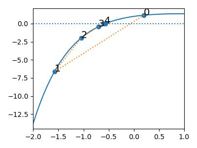
Note that close enough is a very important condition for Newton's method.
Consider \(f(x) = 1 + xe^{-x}\)

def f(x):
    return 1 + x * np.exp(-x)
def df(x):
    return (1 - x) * np.exp(-x)
def Newton(x):
    return x - f(x) / df(x)

iter_ = 5
n1 = [0.2] 
n2 = [1.1]
for i in range(iter_):
    n1.append(Newton(n1[-1]))
    n2.append(Newton(n2[-1]))
pd.DataFrame({
    'n': np.arange(iter_ + 1),
    'start = ' + str(n1[0]): n1,
    'start = '+ str(n2[0]): n2
})

#>>   n  start = 0.2   start = 1.1
#>>   0     0.200000  1.100000e+00
#>>   1    -1.576753  4.214166e+01
#>>   2    -1.045035  4.870894e+16
#>>   3    -0.705991           inf
#>>   4    -0.581505           NaN
#>>   5    -0.567311           NaN

x = np.arange(-2, 5, 0.01)
y = f(x)
plt.figure(figsize=(4, 3))
plt.plot(x, y)
n1 = np.array(n1)
plt.scatter(n1, f(n1))
plt.plot(n1, f(n1), ls=":")
plt.axhline(y=0, ls=":")
for i in range(iter_):
    plt.annotate(str(i), (n1[i], f(n1)[i]), size=14);
plt.xlim(-2, 1)
plt.tight_layout()
plt.savefig("assets/non_linear_equations_3.jpg")

Secant Method

Note that when \(f'(x) = 0\) and \(f(x)\neq 0\), things get somewhat messy with Newton's method. Also, computing derivative is not convenient/possible in all cases.

Consider the approximation of \(f'(x_n)\) by \(\frac{f(x_n) - f(x_{n-1})}{x_n - x_{n-1}}\), then we have

Note that secant method will have the same issue as Newton's method for the convergence

def secant(l, f):
    nomi = f(l[-1]) * (l[-1] - l[-2])
    denom = f(l[-1]) - f(l[-2])
    l.append(l[-1] - nomi / denom)

l = [-1.5, 0.2]
for i in range(5):
    secant(l, f)
l = np.array(l)
plt.figure(figsize=(4, 3))
plt.plot(x, f(x))
plt.scatter(l, f(l))
plt.plot(l, f(l), ls=":")
plt.axhline(y=0, ls=":")
plt.xlim(-2, 1)
for i in range(7):
    plt.annotate(str(i), (l[i], f(l)[i]), size=14)
plt.tight_layout()
plt.savefig("assets/non_linear_equations_4.jpg")

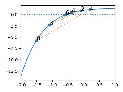
It is proven that the rate of convergence is \(r = \frac{1+\sqrt 5}{2}\approx 1.618\), so that it is slower than Newton's method.