LU Decomposition

import numpy as np
import matplotlib.pyplot as plt
import seaborn as sn

Note that

\[Ax = b \Rightarrow M_{n-1}...M_2M_1Ax = M_{n-1}...M_2M_1b = \hat b\]

\(M_i\) are \(n\times n\) matrices,

Let \(U = M_{n-1}...M_1A\) where \(U\) is upper triangular. Then \(Ux = \hat b \Leftrightarrow Ax = b\) and since \(U\) is triangular, it's very easy to solve \(Ux = \hat b\) (bottom up). Note that \(U\) must have all its diagonal being non-zero.

Note that for each row, it takes \(1\) division and \(n\) multiplications and \(n\) additions. There's a total of

\[n\cdot \text{DIV} + \sum^n (i - 1)(\text{ADD} + \text{MULT}) = n\cdot \text{DIV} + \frac{n(n-1)}{2}(\text{ADD}+\text{MULT})\]

Gaussian Elimination

Denote the entries of all matrices in such

\[A = \begin{bmatrix}a_{11}&...&a_{1n}\\...&...&...\\a_{n1}&...&a_{nn}\end{bmatrix}\]

Consider \(M_1\) so that \(M_1A\) have the first column be \((a_{11}, 0, ..., 0)^T\). Let the diagonal of \(M_1\) be all \(1\), and the first column be \(m_{i1}=-\frac{a_{i1}}{a_{11}}, i = 1, 2,..,n\) (note that \(m_{11}=a_{11}/a_{11}=1\)).

\[M_1 = I - \vec m_1\vec e_1^T, \vec m_1 = (0, \frac{a_{21}}{a_{11}}, ..., \frac{a_{n1}}{a_{11}})\]

Then, for \(M_2\), \(M_2A\) have the first two columns be \((a_{12}, a_{22}, 0, ..., 0)^T\). Let \(M_2\) be the identity with the second column be \(m_{i1}=-\frac{\hat a_{i2}}{a_{22}}, i = 2, 3,...,n\)

\[M_2 = I - \vec m_2\vec e_2^T, \vec m_2 = (0, 0, \frac{a_{32}}{a_{22}}, ..., \frac{a_{n2}}{a_{22}})\]

Therefore, we are recursively doing Gaussian elimination, and each time, we reduced one column and shrink the dimension by one.

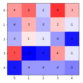
D = 5
M = []
A = np.random.randint(-10, 10, (D, D))
fig, ax = plt.subplots(figsize=(4, 4))
ax.imshow(A,cmap="bwr", vmin=-10, vmax=10)
for (j,ii),label in np.ndenumerate(np.round(A, 2)):
    ax.text(ii,j,label,ha='center',va='center', color="black")
plt.tight_layout()
fig.savefig("assets/lu_decomposition_1.jpg")

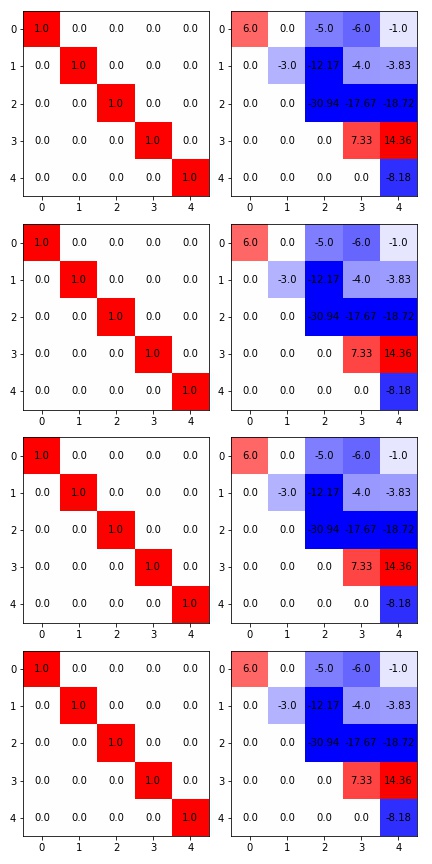
fig, axs = plt.subplots(D - 1, 2, figsize=(6, D*2.4))
for i in range(D - 1):
    m = np.identity(D)
    m[i+1:, i] -= A[i+1:, i] / A[i, i]
    A = m @ A
    axs[i][0].imshow(m, cmap="bwr", vmin=-1, vmax=1)
    for (j,ii),label in np.ndenumerate(np.round(m, 2)):
        axs[i][0].text(ii,j,label,ha='center',va='center', color="black")
    axs[i][1].imshow(A, cmap="bwr", vmin=-10, vmax=10)
    for (j,ii),label in np.ndenumerate(np.round(A, 2)):
        axs[i][1].text(ii,j,label,ha='center',va='center', color="black")
plt.tight_layout()
fig.savefig("assets/lu_decomposition_2.jpg")

Total work

Division: \((n-1) + (n-2) + ... + 1 = \frac{n(n-1)}{2}\)
Multi and Add: \((n-1)^2 + (n-2)^2 + ... + 1 = \frac{n(2n-1)(n-1)}{6}\)
Total: \(\frac{n^3}{3} + O(n^2)\)

Compute b hat

\[\hat b = M_{n-1}...M_{1}b\]

Note that matrix matrix multiplication \(M_iM_j\) takes \(O(n^3)\) operations while matrix vector multiplication \(M_ib\) takes \(O(n^2)\) operations.

Also, note that \(M_1 = I - m_1e_1^T\),

\[M_1b = b - (\vec m_1e_1^Tb) = b - \vec m_1(e_1^Tb) = b - \vec m_1b_1\]

Only takes \(n-1\) additions and multiplications

Similarly,

\[M_2M_1b = M_2\tilde b = \tilde b - m_2\tilde b_2\]

Takes \(n-2\) additions and multiplications

The total steps are \(\frac{n(n-1)}{2} = \frac{n^2}{2} + O(n)\) addition and multiplications

If we want to solve \(Ax = b, Ay = c\), we can store \(M_{n-1}...M_1A\) so that we only have to compute \(\hat b, \hat c\) which takes much less time. (Since the most expensive work is to get \(M_k\)'s).

Properties of M's

Note that determinant of triangular matrices are the product of the diagonal See Proof

Therefore, \(M\) are non-singular with \(det(M)=1\)

Theorem \(M_1^{-1} = (I + m_1e_1^T)\)

proof.

\[\begin{align*} MM_1^{-1} &= (I-m_1e_1^T)(I+m_1e_1^T) \\ &= I - Im_1e_1^T + Im_1e_1^T + (m_1e_1^T)(m_1e_1^T)\\ &= I - m_1(e_1^Tm_1)e_1^T\\ &= I - m_1\quad [1,0,...,0]\begin{bmatrix}0\\m_{21}\\...\\m_{n1}\end{bmatrix}\quad e_1^T\\ &= I - m_10e_1^T\\ &= I \end{align*}\]

LU Factorization

Want to find \(L\) being lower triangular and \(U\) upper triangular so that \(A = LU\).

By Gaussian elimination we already have \(U\) so that we can have \(A = M_1^{-1}...M_{n-1}^{-1}U\), so that \(L = M_1^{-1}...M_{n-1}^{-1}\)

By theorem above, we know \(M_k = I-m_ke_k^T\)

Note that \(M_1^{-1}...M_{n-1}^{-1} = I + \sum_{i=1}^N m_ie_i^T\)

If you have a LU factorization of \(A\), then can easily solve \(Ax=b\Rightarrow LUx = b \Rightarrow Ly = b\)
So that we can solve \(Ly=b\) then \(Ux=y\)

Runtime

Since \(L\) is lower triangular. we'll solve top down, and takes a total of \(\frac{n(n-1)}{2}\) addition and multiplication.

Computing Determinant

Consider \(A_{kk}\) be \(A_{k:n \times k:n}\) so that the classical way of solving determinant will be expanding the determinant along a row/column

\[\det(A) = \sum_{i=1}^n (-1)^{i-1}{a_{1i}} \det(A_{ii})\]

Let \(t(n)\) be the number of multiplications to compute \(A_{n\times n}\) then \(f(n)=nf(n-1) +n \geq n!\)

Theorem \(\det(AB) =\det(A)\det(B)\)

So that \(\det(A) = \det(L)\det(U) = 1 \times diag(U)\)
Remember that computing \(U\) takes \(\frac{n^3}{3} + O(n^2)\) times