Interpolations
Introduction
For a given sequence of observations \(\{(x_i, y_i)\}^n_{i=1}\), we want to find some \(f:\mathbb R\rightarrow \mathbb R\) s.t. \(f(x_i) = y_i\) or in some cases \(f(x_i) \approx y_i\). The approximation can be defined as Least square approximation \(\arg\min_f\|f(x_i) - y_i\|\), where \(f\) belongs to some group of functions (say we want to fit a line).
Usages in Numerical Methods
- Newton's method
- Integrals: for some \(f\) that is hard to find integral, find some polynomial \(p\rightarrow^{p.w.} f\).
Polynomial Interpolations
Given \(\{(x_i,y_i)\}_{i=1}^n\), WTF \(f(x) = \sum_{i=1}^n c_i \phi_i(x)\), i.e.
If \(A\) is nonsingular, then always a unique solution to \(f(x_i) = y_i\)
Monomial Basis
If we let \(\phi_i(x) = x^{i-1}\), then \(f(x) = p(x) = \sum_{i=0}^N c_i x^i\) s.t. \(p(x_i) = y_i\) and we have
Note that \(A\) is non-sigular if \(x_i\)'s are distinct.
Proposition Given \(A\) is non-singular, then \(Ac =0\) IFF \(c=0\)
proof. Define \(p(x_j) := \sum_{i=1}^n c_i x_j^{i-1} = 0\) for \(j = 1,...,n\). \(p(x)\) is a polynomial of degree \(n-1\).
By fundamental theorem of algebra, if at least one \(c_i \neq 0\) then \(p(x)\) has at most \(n-1\) roots.
Example
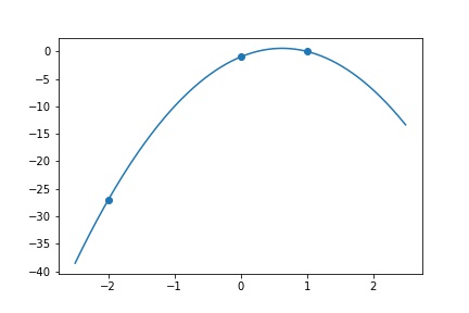
Find a quadratic \(p(x) = c_1 + c_2 x + c_3 x^2\) s.t. \(p(-2) = -27, p(0) = -1, p(1) = 0\) Then we construct \(A = \begin{bmatrix} 1&(-2)^1&(-2)^2\\1&0&0^2\\1&1&1^2\end{bmatrix} = \begin{bmatrix} 1&-2&4\\1&0&0\\1&1&1\end{bmatrix}, y = \begin{bmatrix}-27\\-1\\0\end{bmatrix}\)
x = np.array([-2, 0, 1])
y = np.array([-27, -1, 0])

def find_fit(x, y):
    A = np.empty((x.shape[0], x.shape[0]))
    for i in range(A.shape[0]):
        A[:, i] = x ** i
    c = np.linalg.solve(A, y)
    return c
c = find_fit(x, y)
print("y = " + " + ".join([str(int(round(c[i]))) + "x^" + str(i) for i in range(c.shape[0])]))
#>> y = -1x^0 + 5x^1 + -4x^2
xl = np.arange(-2.5, 2.5, 0.01)
yl = sum([c[i] * (xl ** i) for i in range(c.shape[0])])
plt.plot(xl, yl)
plt.scatter(x, y)
plt.savefig("assets/interpolations_1.jpg")

Conditioning
Often Vandermonde Matrices are very badly conditioned. When \(x_1\neq x_2\) but \(x_1\approx x_2\), then first two rows of \(A\) are almost identical, resulting close to singular and bad conditioning.
Properties of Polynomials
- easy differentiation and integral
- efficient evaluation
We can evaluate by
Or we can even improve by noticing that \(p(x) = c_0 + c_1x + c_2x^2 = c_0 + (c_1 + x(c_2 + x))\)
Lagrange Form of the Interpolation Polynomial
WTF \(p(x_i) = y_i\) for \(i = 1, 2,...,n\) and \(p\) has \(n-1\) degree. \(x_i\) are distinct.
Define the Lagrange basis functions
Note that \(l_j(x_i) = \mathbb I(i=j)\) Then \(p(x) = \sum_{j=1}^n l_j(x)y_j\)
Note that for each \(l(x)\), there are at most \(n-1\) times of \(x\) multiplied together, hence at most \(n-1\) degree.
Consider \(p(x_i) = \sum l_j(x)y_j\), because the indicator property of \(l\), only \(i_i(x_i) = 1\) and others are all 0, therefore, the result is \(l_i(x) y_i + \sum_{j\neq i} l_j(x)x_j = y_i + \sum 0 = y_i\)
Given the same example \(p(-2) = -27, p(0) = -1, p(1) = 0\)
def indicator(x, j, x_array):
    prod = 1
    for i in range(len(x_array)):
        if i != j:
            prod *= ((x - x_array[i]) / (x_array[j] - x_array[i]))
    return prod

def p_lagrange(x, x_array, y_array):
    ret = 0
    for i in range(len(x_array)):
        ret += indicator(x, i, x_array) * y_array[i]
    return ret

yl = []
for e in xl:
    yl.append(p_lagrange(e, x, y))

plt.plot(xl, yl)
plt.scatter(x, y)
plt.savefig("assets/interpolations_2.jpg")
Consider the equation \(p(x) = \sum l_i(x)c_i\), which the problem becomes the system of equations
Now, consider the property of \(l\), only the diagonal \(l_i(x_i) = 1\), i.e. \(A = I, c_i = y_i\).
Computation
Need almost no time to construct, while it's hard to use.
Newton Form of Interpolation Polynomials
Basis Function
Let \(\pi_1(x) = 0, \pi_j(x) = \prod_{i=1}^{j-1}(x-x_i)\) for \(j \geq 2\)
Let \(p_j(x) = \sum_{i=1}^j c_i \pi_i(x)\).
Assuming we have found \(c_j\)'s s.t. \(p_j(x_i) = y_i\) for \(i\in\{1,...,j\}\) and we want to find \(c_{j+1}\) so that \(p_{j+1}(x) := p_t(x) + c_{j+1}\pi_{j+1}(x)\) and \(p_{j+1}(x_i) = y_i\) for \(i\in \{1,...,j+1\}\)
Consider such recurrence relationship, \(\forall i < j+1, \pi_{j+1}(t_i) = 0\) (since one of \((x-x_i)\) in \(\pi\) must be 0).
So that
Define some \(y\) such that the following relationship holds
Define the divided difference table
| \(y[t_i]\) | \(y[t_i, t_{i+1}]\) | \(y[t_i, t_{i+1}, t_{i+2}]\) | \(y[t_i, t_{i+1}, t_{i+2}, t_{i+3}]\) | |
|---|---|---|---|---|
| \(t_1\) | \(y[t_1] = y_1\) | \(y[t_1, t_2] = \frac{y[t_2] - y[t_1]}{t_2 - t_1}\) | \(y[t_1, t_2, t_3] = \frac{y[t_2, t_3] - y[t_1, t_2]}{t_3 - t_1}\) | \(y[t_1, t_2, t_3, t_4] = \frac{y[t_2, t_3, t_4] - y[t_1, t_2, t_3]}{t_4 - t_1}\) |
| \(t_2\) | \(y[t_2] = y_2\) | \(y[t_2, t_3] = \frac{y[t_3] - y[t_2]}{t_3 - t_2}\) | \(y[t_2, t_3, t_4] = \frac{y[t_3, t_4] - y[t_2, t_3]}{t_4 - t_2}\) | |
| \(t_3\) | \(y[t_3] = y_3\) | \(y[t_3, t_4] = \frac{y[t_4] - y[t_3]}{t_4 - t_3}\) | ||
| \(t_4\) | \(y[t_4] = y_4\) |
And we will use the first row to compute \(c_j\)'s.
Such table needs around \(n^2/2\) operations
Such divided difference table actually approximates the \((n+1)\)th derivative.
Computation
Therefore, for each iteration, \(1\) adds and \(2\) multiplications are performed. Where a total of \(n-1\) iterations are needed.
Error of Interpolations
Suppose \(y_i = y(t_i)\) for some smooth function \(y\), i.e. \(y_i\) are coming out of some underlying function model \(y\). We aim to measure \(\|y-p\|_\infty\)
Claim
where \(\epsilon_t\) is in the smallest interval containing \(t_1,...,t_n\)
Recall Rolle's Theorem Given continuous \(\phi'(t). \phi(t_1) = \phi(t_2) = 0\Rightarrow \alpha \in (t_1, t_2). \phi'(\alpha) = 0\)
proof. Fix \(t\). Define \(w(t) = \prod (t-t_i)\)
Suppose \(t\in \{t_i\}\). Then \(y_{t_i} - p(t_i) = 0\land \prod (t - t_i) = 0\) (one of it is 0).
Suppose \(t\not\in \{t_i\}\), define function
Then \(\phi(t)=0\) and we have \(n+1\) distinct places where \(\phi(s)=0\), hence \(n\) places where \(\phi'(s) = 0\), ... \(1\) place where \(\phi^{(n)}(s) = 0\) Notice that
However, \(p\) is a polynomial of degree \(n-1, p^{(n)}(s) = 0\)
\(w(s) = \prod^n (s-t_i) = s^n + o(s^{n-1})\Rightarrow w^{(n)}(s) = n!\)
Therefore
Let \(\phi^{(n)}(s) = 0, y(t)-p(t) = \frac{w(t)y^{(n)}(s)}{n!}\) as required
Consider the Taylor expansion of \(y\), with Taylor's remainder and centered at \(t_1\), i.e. \(y(t) = \sum^n \frac{y^{(i)}(t) (t-t_1)}{(n-1)!} + \frac{y^{(i)}(\epsilon) (t-t_1)}{(n-1)!}\) and \(p\) is now equal to the Taylor polynomial.
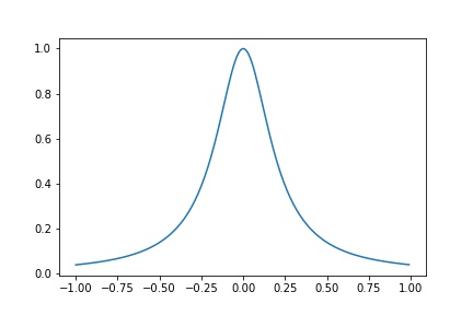
Polynomial Interpolations does not always converge
Consider Runge's Function \(y(t) = (1+25 t^2)\). Taken #n# evenly spaced points on \([-1,1]\) and interpolate \(y(t)\) by a polynomial. However, \(y(t)-p(t)\) does not converges.
x = np.arange(-1, 1, 0.01)
y = 1/(1 + 25 * (x**2))
plt.plot(x, y)
plt.savefig("assets/interpolations_3.jpg")
Piece-wise Polynomial Interpolation
If we take several polynomials and assign each to a domain.
Piece-wise linear polynomials
Suppose we want to interpolate on \([a,b]\), partition \([a,b]\) into \(x_0, ..., x_n\). Then, on each interval \([x_i, x_{i+1}]\), we have a linear polynomial \(p_i(x) = \frac{y_{i+1} - y_i}{x_{i+1}-x_i}(x-x_i) + y_i, x\in[x_i, x_{i+1}]\)
Define \(y(x)\) be the underlying function, \(s\) be the collection of all \(p_i\), connected in order. Then