Computer Arithmetic Examples import numpy as np
import matplotlib.pyplot as plt
import math
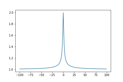
Example 1 Is \(y=\sqrt{1+x^2} - 1=:f(x)\) well-conditioned?
\[\begin{align*} C.N &= \frac{xf'(x)}{f(x)}\\ &= \frac{x(x(1+x^2)^{-1/2}}{(1+x^2)^{1/2}-1}\\ &= \frac{x(x(1+x^2)^{-1/2}}{(1+x^2)^{1/2}-1} \frac{\sqrt{1+x^2}+1}{\sqrt{1+x^2}+1}\\ &= \frac{x^2\sqrt{1+x^2}+1}{\sqrt{1+x^2}(1+x^2-1)}\\ &= \frac{\sqrt{1+x^2} + 1}{\sqrt{1+x^2}}\\ C.N. &\in [1,2] \end{align*}\]
a = np . arange ( - 100 , 100 , 1 )
b = (( a ** 2 + 1 ) ** 0.5 + 1 ) / (( a ** 2 + 1 ) ** 0.5 )
plt . plot ( a , b )
plt . savefig ( "assets/arithmetic_examples_1.jpg" )
Does \(fl(\sqrt{1+x^2}-1)\) always give an accurate result
When \(x\) is small enough so that \(fl(\sqrt{1+x^2}) = 1\) , then \(\hat y = 0, y \neq 0\Rightarrow \frac{\hat y - y}{y}=\infty\) \(fl(\sqrt{1+x^2})=1\Rightarrow x^2 < \frac{\epsilon}{2}\Rightarrow |x|\leq \sqrt{\epsilon/2}\)
When \(|x|\leq \sqrt{\epsilon/2}, x\neq 0\) , this operation gives an inaccurate result, and for moderately small \(x\) this is still not so accurate
Can we change \(\sqrt{1+x^2}-1\) to a mathematically equivalent that has a much smaller f.p. error.
\[(*)=\sqrt{1+x^2}-1\frac{\sqrt{1+x^2}+1}{\sqrt{1+x^2}+1}= \frac{x^2}{\sqrt{1+x^2}+1}\]
lemma 1 \(\sqrt{1+\delta} = 1+\hat \delta, |\hat\delta| < \epsilon/2\) lemma 2 \((1+\delta)^{-1} = 1+\hat\delta, |\hat\delta| < \frac{1.01\epsilon}{2}\)
Claim accuracy
\[\begin{align*} fl\bigg(\frac{x^2}{\sqrt{1+x^2}+1}\bigg) &= (1+\delta_5)\bigg(\frac{x^2(1+\delta_1)}{(\sqrt{(1+x^2(1+\delta_1))(1+\delta_2)}(1+\delta_3)+1)(1+\delta_4)}\bigg)\\ &= \frac{(1+\delta_5)x^2(1+\delta_1)}{[\sqrt{(1+x^2)(1+\hat\delta_1)(1+\delta_2)}(1+\delta_3)+1](1+\delta_4)}\\ &= \frac{(1+\delta_5)x^2(1+\delta_1)}{[\sqrt{(1+x^2)}\sqrt{(1+\hat\delta_1)}\sqrt{(1+\delta_2)}(1+\delta_3)+1](1+\delta_4)}\\ &= \frac{(1+\delta_5)x^2(1+\delta_1)}{[\sqrt{(1+x^2)}(1+\hat\delta_1)(1+\hat\delta_2)(1+\delta_3)+1](1+\delta_4)}\\ &= \frac{(1+\delta_5)x^2(1+\delta_1)}{[\sqrt{(1+x^2)}(1+\tilde\delta_1)(1+\tilde\delta_2)(1+\delta_3)+1](1+\delta_4)}\\ &= \frac{x^2}{\sqrt{(1+x^2)}+1}\frac{(1+\delta_1)(1+\delta_5)}{(1+\delta_1^*)(1+\delta_2^*)(1+\delta_3^*)(1+\delta_4)}\\ &= \frac{x^2}{\sqrt{(1+x^2)}+1}(1+\delta_1)(1+\delta_5)(1+\delta_1^{**})(1+\delta_2^{**})(1+\delta_3^{**})(1+\delta_4^{**}) \end{align*}\]
Note that \(\delta^{**} \leq 1.01\epsilon/2\) , let the product of all \((1+\delta)\) 's, i.e. \(1 + \tilde\delta \leq \frac{7(1.01)\epsilon}{2}\)
\(2.56248\times 10^4, 2.56125\times 10^4\) agrees to 3 sig-dig (to say agree to n sig dit, the exponent must match) \(relative. error = \frac{2.56248 - 2.56125}{2.56125} = \frac{.00123}{2.56125}=1.23/2.56125\times 10^{-3}\) \(p\) sig-dig agree \(\Rightarrow 10^{-p\pm 1}\) relateive error
Example 2 Let \(x = 1\times 10^{-13}, y = 1 + x - 1, z = 4 + x - 4\) \(r_y = (y-x)/x, r_z = (z-x)/x\) will have large relative errors
x = 1.000000000000000000000e-13
y = 1 + x - 1
z = 4 + x - 4
ry = ( y - x ) / x
rz = ( z - x ) / x
print ( "y =" , y )
#>> y = 9.992007221626409e-14
print ( "z =" , z )
#>> z = 1.0036416142611415e-13
print ( "ry =" , ry )
#>> ry = -0.000799277837359144
print ( "rz =" , rz )
#>> rz = 0.003641614261141482
Consider a system of \(\beta=10, p = 5\)
\[x = 1.0000 \times 10^{-3}, y = 1 + x - 1 = 1.0010 - 1 = 0.001 = 1.0000\times 10^{-3}\]
will have no error at all
However, if \(\beta = 2\)
\[\begin{align*} fl_2(1+x) &= &1.0000000 \times 2^0 \\ & &+ 0.00..0b_1b_2...b_k...b_{53}\times 2^0 \\ &= 1.0...0b_1b_2...b_k... b_{53} \times 2^0 \\ &\rightarrow 1.0...0b_1b_2...b_k\\ fl_2(1+x - 1) &= 1.0...0b_1b_2...b_k - 1.0000\times 2^0\\ &= 0.0...0b_1b_2...b_k \times 2^0\\ &= b_1.b_2...b_k00...0\times 2^{-n}\\ \text{Note } x &= b_1.b_2b_3...b_kb_{k+1}...b_{53}\times 2^{-n} \end{align*}\]
We lost the last cut of numbers, and its about 3 significant digits
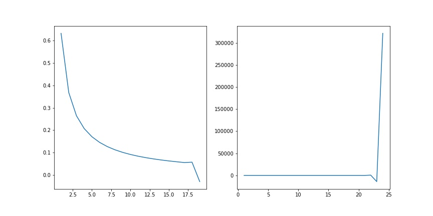
Example 3 Consider the integral \(I_n = \int_0^1 x^n e^{x-1}dx\) , \(n\in \mathbb N\) Note tat \(x^n e^{x-1} > 0, \forall x \in (0, 1), I_n > 0\) \(x^ne^{x-1} > x^{n+1}e^{x-1}\) therefore this is a positive monotonic decreasing sequence.
Also, note that
\[\begin{cases}I_0 = [e^{x-1}]^1_0 = 1/e\\ I_n = [x^ne^{x-1}]^1_0 - n\int_0^1 x^{n-1}e^{x-1}dx = 1-nI_{n-1}\end{cases}\]
Therefore we can calculate this recursively
l = [ 1 - 1 / math . e ]
for n in range ( 1 , 24 ):
l . append ( 1 - n * l [ - 1 ])
fig , axs = plt . subplots ( 1 , 2 , figsize = ( 12 , 6 ))
axs [ 0 ] . plot ( range ( 1 , 20 ), l [: 19 ])
axs [ 1 ] . plot ( range ( 1 , 25 ), l );
fig . savefig ( "assets/arithmetic_examples_2.jpg" )
\[\begin{align*} \tilde I_0 &= I_0 + \epsilon_0, |\epsilon_0| \approx 10^{-16}\\ \tilde I_1 &= 1 - 1 \tilde I_0 = 1 - (I_0 + \epsilon_0) = I_1 - \epsilon_0 \\ \tilde I_2 &= 1 - 2(I_1 - \epsilon_0) = 1 - 2I_1 + 2\epsilon_0 = I_2 + 2\epsilon_0\\ &...\\ \tilde I_n &= I_n + n! \epsilon_0 \end{align*}\]
print ( "n = 10 =>" , 1e-16 * math . factorial ( 10 ))
#>> n = 10 => 3.6288e-10
print ( "n = 18 =>" , 1e-16 * math . factorial ( 18 ))
#>> n = 18 => 0.6402373705728
Consider
\[I_n = 1-nI_{n-1}\equiv I_{n-1} = \frac{1 - I_n}{n}\]
\[\tilde I_{n-1} = \frac{1}{N}(1 - \tilde I_N) = \frac{1 - I_N}{n} - \frac{\epsilon_N}{N}\]
Note that
\[\tilde I_{n-k} = I_{N-k} + (-1)^n \frac{\epsilon_N}{N! / (N-k+1)!}\]
Also, note that \(e^{-1} \leq e^{x-1}\leq e^0 = 1\)
\[\frac{e^{-1}}{n+1}=e^{-1}\int_0^1 x^n dx\leq \int_0^1 x^ne^{x-1}dx \leq \int_0^1 x^ndx = (n+1)^{-1}\]
So that
\[\int_0^1 x^n e^{n-1}dx \approx \frac{1}{2}\frac{1 - e^{-1}}{n+1}\]
\[|I_n - A|\leq \frac{1}{2}(\frac{1 - e^{-1}}{n+1}) = \frac{1}{n+1}\frac{1-e^{-1}}{2}\]
May 6, 2023 January 9, 2023