Support Vector Machines and Boosting

Support Vector Machines

General Setting

If we use \(t\in\{-1, 1\}\) instead of \(\{0,1\}\), i.e. the model is

\[z=\vec w^T\vec x + b, y = sign(z)\]

Hinge Loss

\[\mathcal L_H(z,t) =\max\{0,1-zt\}\]

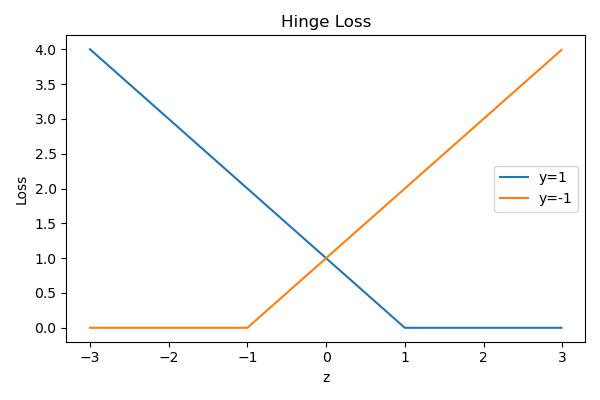
If we use a linear classifier and write \(z^{(i)}(w,b)=\vec w^T\vec x + b\), then we want to minimize the training loss

\[\min_{\vec w, b} \sum_{i=1}^NL_H(z^{(i)}, t^{(i)}) = \min_{\vec w, b} \sum_{i=1}^N \max\{0, 1 - t^(i)z^{(i)}(\vec w, b)\}\]

This formulation is called support vector machines.

Generally used with \(L_2\) regularization

\[\min_{\vec w, b} \sum_{i=1}^N \max\{0, 1 - t^(i)z^{(i)}(\vec w, b)\} + \frac{\lambda\|\vec w\|_2^2}{2}\]

Optimal Separating Hyperplane

Suppose we want to find a linear classifier that separates a set of data points. In \(\mathbb R^2\), this will looks like a line \(y=wx+b\); in \(\mathbb R^{D>2}\), that will be a hyperplane.

Note that there are multiple separating hyperplanes, i.e. different \(w,b\)'s

A hyperplane that separates two classes and maximizes the distance to the closest point from either class, i.e. maximize the margin of the classifier.

Boosting

Train classifiers sequentially, each time focusing on training data points that were previously misclassified.

Key Idea

learn a classifier using different costs (by applying different weights). Intuitively, "tries harder" on examples with higher cost.

Let misclassification rate be and change cost function

\[\frac{1}{N}\sum_{n=1}^N \mathbb I[h(x^{(n)})\neq t^{(n)}] \Rightarrow \frac{1}{N}\sum_{n=1}^N w^{(n)}\mathbb I[h(x^{(n)})\neq t^{(n)}]\]

\(w^{(n)}\) is normalized so that the overall weights does not change the overall loss.

\[\forall n. w^{(n)} > 0, \sum_{n=1}^N w^(n)=1\]

Weak Learner / Classifier

Weak learner is a learning algorithm that outputs a hypothesis that performs slightly better than chance i.e. error rate \(>0.5\)

We want such classifiers for they are computationally efficient.

For example, Decision Stump: A decision tree with a single split.

One single weak classifier is not capable of making the training error small. so that

\[err = \sum_{n=1}^N w^{(n)}\mathbb I[h(x^{(n)})\neq t^{(n)}] \leq \frac{1}{2} -\gamma, \gamma > 0 \text{ is small}\]

Then, we want to combine many weak classifiers to get a better ensemble of classifiers.

Adaptive Boosting (AdaBoost)

Key steps

At each iteration, re-weight the training samples by assigning larger weights to samples that were classified incorrectly.
We train a new weak classifier based on the re-weighted samples
We add this weak classifier to the ensemble of weak classifiers. This ensemble is the new classifier
Repeat the process

Boosting vs. Bootstrap

Boosting reduces bias by making each classifier focus on previous mistakes.
Bootstrap reduces variance, while keeping bias the same

Algorithm

data \(D_N = \{x^{(n)}, t^{(n)}\}_{n=1}^N, t^{(n)}\in\{-1,1\}\)
A classifier or hypothesis \(h: \vec x \rightarrow \{-1, 1\}\)
0 - 1 loss: \(\mathbb I(h(x^{(n)}\neq t^{(n)})) = \frac{(1-h(x^{(n)})t^{(n)})}{2}\)
WeakLearn\(:D_N\times \vec w\rightarrow h\) be a function that returns a classifier

AdaBoost(\(D_N\), WeakLearn):

init \(w^{(n)} = N^{-1}, \forall n\)
For \(t = 1, ..., T\)
- \(h_t\leftarrow \text{WeakLearn}(D_N, \vec w)\)
- compute weighted error \(err_t = \frac{\sum_1^N w^{(n)\mathbb I(h_t(x^{(n)})\neq t^{(n)})}}{\sum_{n=1}^Nw^{(n)}}\)
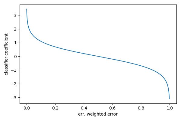
- compute classifier coefficient \(\alpha_t = \frac{1}{2}\log(\frac{1-err_t}{err_t}), a_t \in (0, \infty)\)
- update data weights \(w^{(n)}\leftarrow w^{(n)}\exp(-\alpha_tt^{(n)}h_t(\vec x^{(n)}))\)
return \(H(x) = sign(\sum_{t=1}^T \alpha_t h_t(\vec x))\)

Intuition

Weak classifiers which get lower weighted error get more weight in the final classifier.
Consider the shape of \(\alpha_t\) - If \(err\approx 0, a_t\) high so misclassified examples get more attention - If \(err\approx 0.5, a_t\) low so misclassified examples are not emphasized

Geometric converge

Assume that at each iteration of AdaBoost the WeakLearn returns a hypothesis with error \(err\leq \frac{1}{2} - \gamma\) for all \(t = 1, ..., T\) with \(\gamma > 0\). The training error of the output hypothesis \(H(\vec x) = sign(\sum^T a_th_x(\vec x))\) is at most

\[L_N(H) = \frac{1}{N} \sum^N \mathbb I\{H(\vec x^{(i)}\neq t^{(i)})\}\leq \exp(-2\gamma^2T)\]

under the assumption that weak learner is \(\gamma\)-better than a random predictor.

Additive Model

With a more complex \(H\) by adding more weak classifiers, we expect more complex classifiers overfit. However, this is not often true, sometimes the test error decreases even after the training error is zero.

General Setting

Consider a hypothesis class \(\mathcal H\) with each \(h_i\in\mathcal H:\vec x\rightarrow \{-1,1\}\) being "weak learners", or bases.

Define an additive model with \(m\) terms to be

\[H_m(x) = \sum_{i=1}^m \alpha_ih_i(\vec x)\]

where \((\alpha_1, ..., \alpha_m) \in \mathbb R^m\) and generally \(a_i\in\mathbb R^+, \sum a_i = 1\). So that \(H_m\) is a linear combination of bases classifiers, like in boosting.

Stage-wise Training

Consider a greedy approach to fitting additive models, known as stagewise training

init \(H_0(x)= 0\)
For \(m=1,..., T\)
- compute the \(m\)-th hypothesis \(H_m = H_{m-1} + a_mh_m\) so that the loss is minimized, i.e.
\[h_m,\alpha_m \rightarrow arg\min_{h\in\mathcal H, \alpha\in\mathbb R}\sum_{i=1}^N \mathcal L(H_{m-1}(x^{(i)}) + \alpha h(x^{(i)}, t^{(i)}))\]
- \(H_m = H_{m-1} + \alpha_mh_m\)

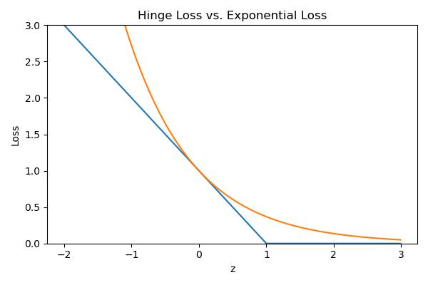
Then consider the exponential loss, as a smooth simulation to Hinge loss.

\[\begin{align*} (h_m,a_m)\leftarrow arg\min &\sum_{i=1}^N \exp(-\bigg[H_{m-1}(x^{(i)} + ah(x^{(i)}))\bigg]t^{(i)})\\ = &\sum_{i=1}^N \exp(-H_{m-1}(x^{(i)}t^{(i)}))\exp(-ah(x^{(i)}t^{(i)}))\\ = &\sum_{i=1}^N w_i^{(m)}\exp(-ah(x^{(i)}t^{(i)})) \end{align*}\]

where \(w_i^{(m)}:= \exp(-H_{m-1}(x^{(i)})t^{(i)})\)

Then, notice that \(h(x)\in \{-1, 1\}\) is the classifier so that

\[h(x^{(i)}) = t^{(i)}, \exp(-ah(x^{(i)})t^{(i)}) = \exp(-a)\]

\[h(x^{(i)}) \neq t^{(i)}, \exp(-ah(x^{(i)})t^{(i)}) = \exp(a)\]

Then, our additive model is equivalent to

\[\begin{align*} \sum_{i=1}^N w_i^{(m)} \exp(-ah(x^{(i)})t^{(i)}) &= e^{-a} \sum^N w_i^{(m)}\mathbb I\{h(x^{(i)})=t^{(i)}\} \\ &+e^a \sum_{i=1}^N w_i^{(m)}\mathbb I(h(x^{(i)})\neq t^{(i)})\\ &= \text{correct predictions + incorrect predictions} \end{align*}\]

Thne, define \(I_{t}=\mathbb I(h(x^{(i)}) = t^{(i)}), I_{f}=\mathbb I(h(x^{(i)}) \neq t^{(i)})\), and consider of summation above, we can further group them by

\[\begin{align*} &e^{-a}\sum^N w_i^{(m)} I_t + e^a\sum^N w_i^{(m)}I_f - e^{-a}\sum^N w_i^{(m)}I_f + e^{-a}\sum^N w_i^{(m)}I_f\\ &= (e^a - e^{-a})\sum_{i=1}^N w_i^{(m)}I_f + e^{-a}\sum_{i=1}^N w_i^{(m)}(I_f+I_t)\\ &= (e^a - e^{-a})\sum_{i=1}^N w_i^{(m)}I_f + e^{-a}\sum_{i=1}^N w_i^{(m)} \end{align*}\]

To optimize \(h\), is equivalent to minimize

\[ (e^a - e^{-a})\sum_{i=1}^N w_i^{(m)}\mathbb I(h(x^{(i)})\neq t^{(i)})\]

To optimize \(\alpha\), define weighted classification error:

\[err_m = \frac{\sum^N w_i^{(m)}\mathbb I(h_m(x^{(i)})\neq t^{(i)})}{\sum w_i^{(m)}}\]

and with of minimization on \(h\)

\[\begin{align*} &\min_a\min_{h\in\mathcal H} \sum_{i=1}^N w_i^{(m)}\exp(-ah(x^{(i)})t^{(i)})\\\ =&\min_a\bigg\{(e^a-e^{-a})\sum^N w_i^{(m)}I_f + e^{-a}\sum^N w_i^{(m)}\bigg\}\\ \mathcal L=&\min_a\bigg\{(e^a-e^{-a})err_m\sum^N w_i^{(m)} + e^{-a}\sum^N w_i^{(m)}\bigg\} \end{align*}\]

Then consider the derivative, where \(W = \sum^N w_i^{(m)}\),

\[\frac{d\mathcal L}{da} = (e^a + e^{-a})err_m W - e^{-a} W\]

Set to 0

\[\begin{align*} (e^a + e^{-a})err_m &= e^{-a}\\ (e^{2a} + 1)err_m &= 1\\ e^{2a} &= \frac{1-err_m}{err_m}\\ a &= \frac{1}{2}\log(\frac{1-err_m}{err_m}) \end{align*}\]

And for each iteration,

\[\begin{align*} w_i^{(m+1)} &= \exp(-H_m(x^{(i)})t^{(i)})\\ &= \exp(-\big[H_{m-1}(x^{(i)} + a_m h_m(x^{(i)}))\big]t^{(i)})\\ &= \exp(-H_{m-1}(x^{(i)})t^{(i)})\exp(-a_mh_m(x^{(i)}t^{(i)}))\\ &= w_i^{(m)}\exp(-a_mh_m(x^{(i)}t^{(i)})) \end{align*}\]

Source code

import numpy as np
import matplotlib.pyplot as plt

z = np.arange(-3, 3, 0.01)
plt.figure(figsize=(6, 4))
plt.plot(z, np.maximum(0, 1 - z), label="y=1")
plt.plot(z, np.maximum(0, 1 + z), label="y=-1")
plt.title("Hinge Loss")
plt.xlabel("z")
plt.ylabel("Loss")
plt.legend()
plt.tight_layout()
plt.savefig("../assets/svm_hinge_loss.jpg")

err = np.arange(0.001, 0.999, 0.001)
a = np.log((1 - err) / err) / 2
plt.figure(figsize=(6, 4))
plt.plot(err, a)
plt.xlabel("err, weighted error")
plt.ylabel("classifier coefficient")
plt.tight_layout()
plt.savefig("../assets/svm_error.jpg")


z = np.arange(-2, 3, 0.01)
plt.figure(figsize=(6, 4))
plt.plot(z, np.maximum(0, 1-z), label="Hinge")
plt.plot(z, np.exp(-z), label="exponential")
plt.title("Hinge Loss vs. Exponential Loss")
plt.xlabel("z")
plt.ylabel("Loss")
plt.ylim(0, 3)
plt.tight_layout()
plt.savefig("../assets/svm_vs.jpg")