Decision Trees

make prediction by recursively splitting on different attributes according to a tree structure

Internal nodes: test attributes
Branching: attribute values
Leaf: output (predictions)

NOTE - can have repeated attributes, but not the same attribute values - can be imaged as splitting the space into rectangular subspaces

Classification and Regression

Each path from root to a leaf defines a region \(R_m\) of input space, let \(\{(x^{(m_1)}, t^{(m_1)}), ..., (x^{(m_k)}, t^{(m_k)})\}\) be the training examples that fall into \(R_m\)

Classification Tree set leaf value \(y^m\) be the most common value in \(\{t^{(m_1)}, ..., t^{(m_k)}\}\), hence discrete output

Regression Tree set leaf value \(y^m\) be the mean value in \(\{t^{(m_1)}, ..., t^{(m_k)}\}\), hence continuous output

Learning (Constructing) Decision Trees

Note that learning the simplest decision tree which correctly classifies training set is NPC

General Idea

Greedy heuristic start with empty and complete training set by split on the "best" attribute and recurse on subpartitions

Accuracy (Loss) based

Let loss \(L:=\) misclassification rate, say region \(R\rightarrow R_1, R_2\) based on loss \(L(R)\) and the accuracy gain is \(L(R) - \frac{\|R_1\|L(R_1) + \|R_2\|L(R_2)}{\|R_1\| + \|R_2\|}\)

Problem sometimes loss in misclassfication rate will have reduced uncertainty significantly.

Uncertainty based

Low uncertainty: all examples in leaf have same class
High uncertainty: each class has same amount of examples in leaf

Idea use counts at leaves to define probability distributions, and use information theory to measure uncertainty

Entropy

measure of expected "surprise", a.k.a. how uncertain are we of the value of a draw from this distribution

\[H(\vec X) = -E_{X \sim p}[\log_2 p(X)] = -\sum_{\vec x\in X} p(\vec x)\log_2 p(\vec x)\]

Average over information content of each observation
Unit = bits (based on the base of log)
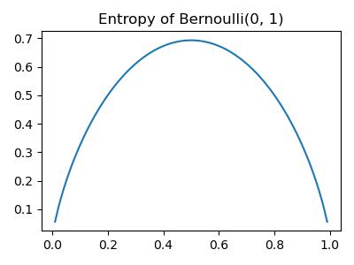
A fair coin flip has 1 bit of entropy, i.e.

\[H(X) = -\frac{1}{2}\log_2 \frac{1}{2} - -\frac{1}{2}\log_2 \frac{1}{2} = -\log_2 \frac{1}{2} = 1\]

Source code

import numpy as np
import matplotlib.pyplot as plt
import scipy.stats as sps

plt.figure(figsize=(4, 3))
x = np.arange(0.01, 1, 0.01)
y = - 1 * x * np.log(x) - (1- x) * np.log(1- x)
plt.plot(x, y)
plt.title("Entropy of Bernoulli(0, 1)")
plt.tight_layout()
plt.savefig("../assets/decision_trees.jpg")

High Entropy

Variable has uniform-ish distribution
Flat histogram
Values sampled from it are less predicatable

Low Entropy

Variable has peaks and valleys
Histogram with low and highs
Values sampled from it are more predicatable

Example

Let X = {Raining, Not raining}, Y = {Cloudy, Not cloudy}

	C	NC
R	24	1
NR	25	50

entropy of a joint distribution

\[\begin{align*} H(X,Y) &= - \sum_{\vec x\in X}\sum_{y\in Y}p(x,y)\log_2 p(x,y)\\ &= -\frac{24}{100}\log_2\frac{24}{100} -\frac{1}{100}\log_2\frac{1}{100}-\frac{25}{100}\log_2\frac{25}{100} -\frac{50}{100}\log_2\frac{50}{100}\\ &\approx 1.56 bits \end{align*}\]

conditional entropy

Given it is raining, what is the entropy of cloudiness

\[\begin{align*} H(Y\mid X = R) &= -\sum_{y\in Y} p(y\mid R)\log_2 p(y\mid R) \\ &= -\frac{24}{25}\log_2\frac{24}{25} -\frac{1}{25}\log_2\frac{1}{25} \\ &\approx 0.24 bits \end{align*}\]

expected conditional entropy

\[\begin{align} H(Y\mid X) &= E_{X\sim p(x)[H(Y\mid X)]} \\ &= \sum_{x\in X}p(x)H(Y\mid X= x) \\ &= - \sum_{x\in X}\sum_{y\in Y}p(x,y)\log_2 p(y\mid x)\\ &= -E_{(X,Y)\sim p(x,y)}[\log_2 p(Y\mid X)] \end{align}\]

What is the entropy of cloudiness, given whether it is raining

\[\begin{align*} H(Y\mid X) = \sum_{x\in X}p(x)H(Y\mid X=x) \\ &= \frac{1}{4}H(Y\mid R) + \frac{3}{4} + H(Y\mid NR)\\ &\approx 0.75 bits \end{align*}\]

Properties

for the discrete case

\(H\geq 0\)
\(H(X,Y)= H(X\mid Y) + H(Y) = H(Y\mid X) + H(X)\)
\(X,Y\) indep. \(\Rightarrow H(Y\mid X) = H(Y)\)
\(H(Y\mid Y) = 0\)
\(H(Y\mid X)\leq H(Y)\)

Information Gain

In \(Y\) due to \(X\) (or mutual information of \(Y\) and \(X\))is defined as

\[IG(Y\mid X) = H(Y) - H(Y\mid X)\]

Since \(H(Y\mid X )\leq H(Y), IG\geq 0\)
\(X\) is completely uninformative about \(Y\Rightarrow IG(Y\mid X)= 0\)
\(X\) is completely informative about \(Y\Rightarrow IG(Y\mid X) = H(Y)\)

Then, foe each decision, we gain some \(X\), so that we can calculate \(IG\)

Algorithm

Start with empty decision tree and complete training set
Split on the most informative attribute (most \(IG\)), partitioning dataset
Recurse on subpartitions
Possible termination condition: end if all examples in current subpartition share the same class

What makes a "Good" tree

Small Tree can't handle important but possibly subtle distinctions in data
Big tree bad computational efficiency, over-fitting, human interpretability

Occam's Razor find the simplest hypothesis that fits the observations

Expressiveness

Discrete input & output case: can express any function of input attributes
Continuous input & output: can approximate any function arbitrarily closely

There's a consistent decision tree for any training set with one path to leaf for each example, while won't generalize to new examples

Miscellany

Problems

exponentially less data at lower levels
Too big tree => overfit
Greedy don't necessarily yield the global optimum
Mistakes at top-level propagate down tree

For continuous attributes, must be split based on thresholds, which is more computational intensive in choosing more parameters

With regression, use MSE as splits instead of IG

Decision Tree vs. kNN

Advantages of Decision Tree

Good with discrete attributes
Easily deals with missing values
Robust to scale of inputs
Test time is fast
More interpretable

Advantages of kNN

Able to handle attributes/feature with interactions in complex ways
Can incorporate interesting distance measures