Fluid Simulation

Generally, there are two approaches for fluid simulation:

Grid approach: discretize the 3D field as a grid and save quantities on voxels, the fluids will move through grid and updates quantities accordingly. Easy to scale, but hard to track the surface.
Particle approach: each particle represents a blob of volume and stores quantities. The fluid behavior is achieved through inter-particle forces. Hard to scale, but easy to track surface.

Grid based Fluid Simulation

For simplicity, assume a 2D simulation, and 3D simulation behaves exactly the same.

For grid-based simulation, we store velocity, pressure, density on a regular grid. Note that pressure and density are scalar fields \(p: \mathbb R^2 \rightarrow \mathbb R\) while velocity is 3D fluid \(\mathbf v: \mathbb R^2\rightarrow\mathbb R^2, \mathbf v(x,y) = (u,v)\).

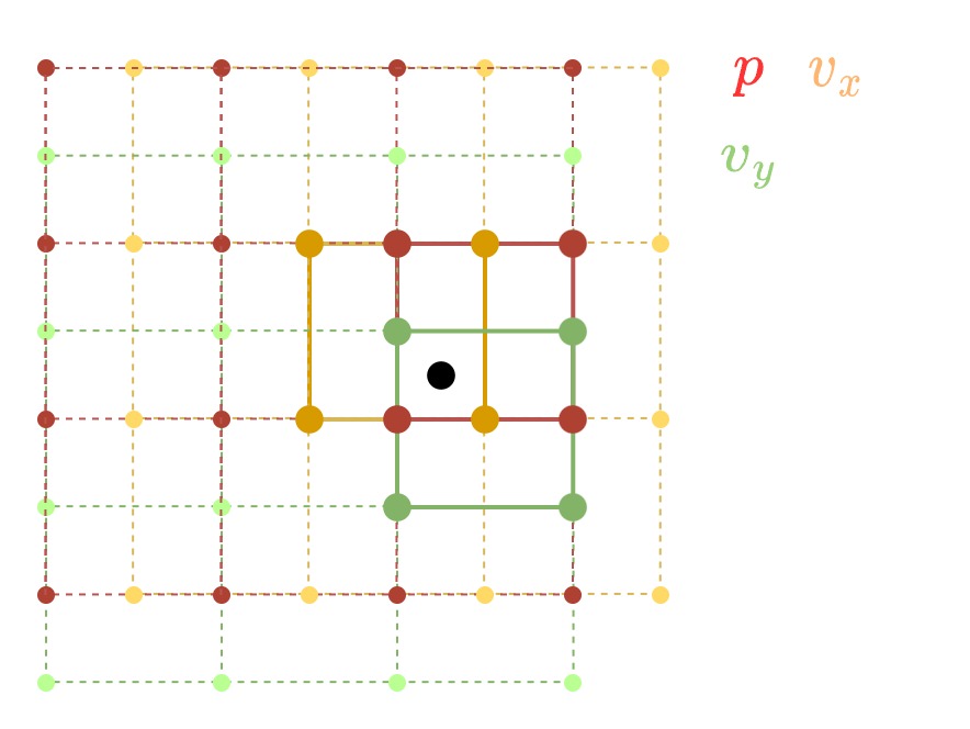
Staggered Grid

Intuitively, we can store all quantities on discretized grid locations, and linearly interpolate the values at any location (lerp from \(2^D\) points), i.e.

\[\begin{align*} p(x,y) &= lerp(p_{i,j}, p_{i+1,j}, p_{i,j+1}, p_{i+1,j+1})\\ \mathbf v(x,y) &= lerp(\mathbf v_{i,j}, \mathbf v_{i+1,j}, \mathbf v_{i,j+1}, \mathbf v_{i+1,j+1})\\ \end{align*}\]

where \(i = \lfloor x / dx \rfloor, j = \lfloor y / dy \rfloor\). However, to prevent unstable checkerboard, we use a staggered grid instead. The pressure grid is unchanged, while the velocity is staggered by half, which means that

\[\begin{align*} i_p &= \lfloor x / dx \rfloor, j_p = \lfloor y / dy \rfloor\\ i_{u} &= \lfloor x / dx + 0.5\rfloor, j_{u} = \lfloor y / dy \rfloor\\ i_{v} &= \lfloor x / dx \rfloor, j_{v}= \lfloor y / dy + 0.5\rfloor \end{align*}\]

Vector Field

Define several operators on the vector field.

gradient for some scalar field \(p\), \(\nabla p = (\partial_x p, \partial_y p)\) is the direction of greatest change in \(p\)
divergence for some field \(\mathbf v:(x,y)\rightarrow(u,v)\), \(\nabla \cdot \mathbf v = \partial_x u + \partial_y v\) is the net flow of the region near \((x,y)\).
curl \(\nabla\times \mathbf v = \partial_xv - \partial_yu\) is the circulation around \((x,y)\).
Laplacian \(\nabla^2 p= \nabla\cdot\nabla p= \frac{\partial^2p}{\partial x^2} + \frac{\partial^2p}{\partial y^2}\) is the difference from the neighborhood average.
directional derivative \(\nabla_{\mathbf v} \mathbf v = \mathbf v \cdot \nabla \mathbf v\) measures how a quantity changes as point of observation moves

Navier-Stokes Equations

The change in fluid velocity is described as

\[\frac{\partial\mathbf v}{\partial t} = -\nabla_{\mathbf v}\mathbf v - \frac{\nabla p}{\rho} + \frac{\nu}{\rho}\nabla^2 \mathbf u + \frac{\mathbf f}{\rho}\]

\(\nabla_{\mathbf v}\mathbf v\) is the advection
\(\frac{\nabla p}{\rho}\) is pressure, \(\rho\) is density
\(\frac{\nu}{\rho}\nabla^2 \mathbf u\) is viscosity, \(\nu\) is the viscosity coefficient
\(\frac{\mathbf f}{\rho}\) is the external forces on the field

This leads to a forward solver

\[d\mathbf v = dt(-\nabla_{\mathbf v}\mathbf v - \frac{\nabla p}{\rho} + \frac{\nu}{\rho}\nabla^2 \mathbf u + \frac{\mathbf f}{\rho})\]

where we update pressure \(p\) from density \(rho\), then update velocities by N-SE, and update densities from \(\dot{\rho} \propto -(\nabla_{\mathbf v}\rho + \nabla\cdot (\rho\mathbf v))\).

However, iteratively solving the equation (explicit method) will quickly go unstable because pressure waves move fast.

Stable Fluids

Stable Fluids [Stam 1999]¹ is an early work that provide a more stable solver for N-SE by making the incompressible assumption.

Incompressible Fluids

We add an additional assumption that the fluid has constant density / volume, which implies that the divergence of flow velocity is \(0\), i.e. \(\nabla\cdot \mathbf v = 0\). Then we separate the problem by taking out advection \(d\mathbf v_a = -dt\nabla_{\mathbf v}\mathbf v\) and pressure projection \(d\mathbf v_p = - dt\frac{\nabla p}{\rho}\). Then, the equation becomes

\[d\mathbf v = d\mathbf v_a + d\mathbf v_p +dt( \frac{\nu}{\rho}\nabla^2 \mathbf u + \frac{\mathbf f}{\rho})\]

We separate problem term \(\mathbf v^*\), the unprojected and unadvected velocities, from the rest

\[\mathbf v^* = \mathbf v^t + dt(\frac{\nu}{\rho}\nabla^2 \mathbf u + \frac{\mathbf f}{\rho})\]

The incompressible fluid assumption gives that

\[\begin{align*} \nabla\cdot\mathbf v &= 0\\ \nabla \cdot(\mathbf v^* + d\mathbf v_p) &= 0\\ \nabla\cdot \mathbf v^* + \nabla\cdot(-dt \frac{\nabla p}{\rho}) &= 0\\ \nabla\cdot\mathbf v^* &= dt \nabla\cdot\frac{\nabla p}{\rho}\\ \nabla\cdot\mathbf v^* &= \frac{dt}{\rho}\nabla^2 p \end{align*}\]

we can now solve \(p\) and unproject pressure back to as \(\mathbf v^+ = \mathbf v^* - \frac{dt}{\rho}\nabla^2 p\).

Finally, we can update advection simply by track backward each velocity \(\mathbf v_{i,j}\) for \(dt\), interpolate the values and copy to new location.

Stam, J. 1999. Stable fluids. Proceedings of the 26th annual conference on computer graphics and interactive techniques, 121–128. ↩