Examples: Equality Constrained Finite Dimension Optimization
Example 1
Question
Show that maximizing logistic likelihood is equivalent to minimizing negative log likelihood.
proof. Note that maximizing \(\mathcal L\) is equivalent to maximizing \(\log(\mathcal L)\) since \(\log\) is a monotone increasing function. Also, minimizing a function's negative is equivalent to maximizing the function.
Denote \(c_i = \exp(a_i^Ty+\beta), d_j = \exp(b_j^Ty+\beta)\). The likelihood for logistic classification is
Then, the negative log likelihood is
Therefore, minimize \(\mathcal L\) is quivalent to maximize \(-\log(\mathcal L)\)
Example 2
Question
Show that polynomial approximation can be written in a quadratic form.
proof. First, the equation is
The first summation is
The second summation term is
Define \(\vec x_k = (1, x_k, x_k^2,...,x_k^{n})\), then then last summation term is
Note that \(\vec x_k \vec x_k^T = Q_k\) where \(q_{k_{ij}} = [x_k^{i+j}]\) and \(\sum_{k=1}^m Q_k = Q\).
Therefore, \(f(a) = a^TQa - 2b^Ta + c\)
Example 3
Question
Find the regular points on \(M = \{(x, y) \in\mathbb R^2\mid (x-1)^2(x-y)(x+y) = 0\}\).
Note that the set of all feasible points are \(\{(x,y)\in\mathbb R^2\mid x=1\}\cup \{(x,y)\in\mathbb R^2\mid x=y\}\cup \{(x,y)\in\mathbb R^2\mid x=-y\}\).
Let \(h(x, y) = (x-1)^2(x-y)(x+y)\), then
Set \(\nabla h(x, y) =0\), we solve \(\begin{cases}-2(x-1)^2y = 0\\4x^3 - 6x^2 - 2xy^2 +2x+2y^2=0\end{cases}\)
For the set \(\{(x,y)\in\mathbb R^2\mid x=1\}\), obtained
solves to be \(y\in\mathbb R\).
For the set \(\{(x,y)\in\mathbb R^2\mid x=y\}\), obtained
solves to have \(x=y=0\) and \(x=y=1\)
For the set \(\{(x,y)\in\mathbb R^2\mid x=-y\}\), obtained
solves to have \(x=y=0\) and \(x=1, y=-1\)
Combine the cases together, we obtained that the regular points are \(\{(x,y)\in\mathbb R^2\mid x= 1\}\cup \{(0, 0)\}\)
Example 4
Question
Consider the minimization problem
Part (a)
Which feasible points are regular.
First, obviously the feasible points are \(\{(0, y, 0)\mid y\in\mathbb R\}\). Also, note that \(\nabla h_1 = (1, 0, 0), \nabla h_2 = (0, 0, 1)\) are always linearly independent. Therefore, all feasible points are regular
Part (b)
Find candidates for minimizer.
First note that \(\nabla f = \begin{bmatrix}2x-y\\2y-x-3\\2z\end{bmatrix}\). Using the Lagrange multipliers method, let \(\lambda_1, \lambda_2 \in\mathbb R\), we obtain the equations
Solve the equations on the constraints \(x=0, z=0\), we have
Which solves to have \(y=2/3, \lambda_1 = 2/3, \lambda_2 = 0\) so that the candidate for minimizer is \((0, 2/3, 0)\)
Part (c)
Check 2nd order condition.
\(\nabla^2 f = \begin{bmatrix}2&-1&0\\-1&2&0\\0&0&2\end{bmatrix}, \nabla^2 h_1 = 0, \nabla^2 h_2 = 0\), \(\nabla^2 f + \lambda_1\nabla^2 h_1 + \nabla^2 h_2 = \nabla^2 f\) is a positive semidefinite matrix on \(\mathbb R^3\), hence also on \(M\). By 2nd order condition, \((0,3/2, 0)\) is a minimizer.
Example 5
Question
Let Q be symmetric \(n\times n\) matrix with eigenvalues \(\lambda_1 \leq ...\leq \lambda_n\) and consider minimize \(f(x)=\frac{x^TQx}{x^Tx}\) subject to \(\sum^n i(x_i^2) = 1\), find the min value in terms of \(\lambda\)'s.
First, note that for any \(x\in\mathbb R^n, a\in\mathbb R\),
Therefore, let \(a = \|x\|^{-1}\), we have \(f(x') = f(\frac{x}{\|x\|})\) so that \(f(x') = \frac{x'^TQx'}{1} = x'^TQx'\) and \(\|x'\| = 1\).
Then, because \(Q\) is symmetric,
Let \(h(x) = \sum_{i=1}^n i(x_i)^2 - 1\), so that
By Lagrange multiplier, take some \(\lambda\in\mathbb R\), and we have
Question 6
Question
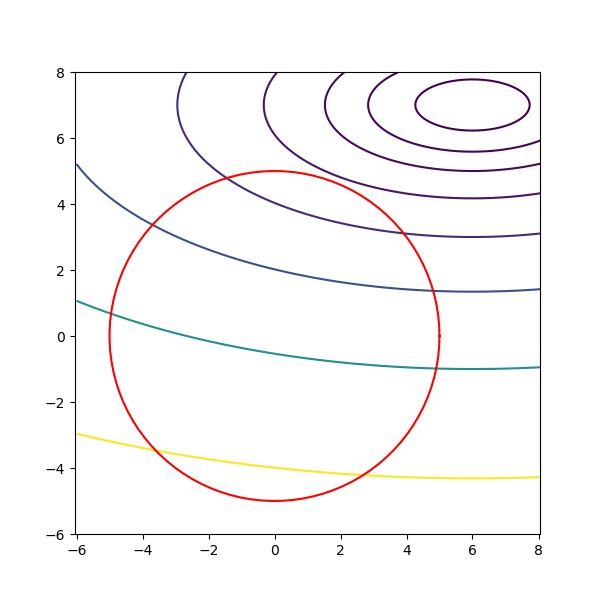
optimize \(f(x,y) = (x-6)^2 + 5(y-7)^2\) subject to \(h(x, y) = x^2+y^2 - 25 =0\).
Source code
import matplotlib.pyplot as plt
import numpy as np

x = np.arange(-6, 10, 0.01)
y = np.arange(-6, 12, 0.01)
xx, yy = np.meshgrid(x, y)
f = (xx - 6) ** 2 + 5 * (yy - 7)**2

plt.figure(figsize=(6, 6))
plt.contour(xx, yy, f, levels=[3, 10, 20, 40, 80, 160, 320, 640])
an = np.linspace(0, 2 * np.pi, 100)
plt.plot(5 * np.cos(an), 5 * np.sin(an), color="red")
plt.axis("equal")
plt.xlim(-6, 8)
plt.ylim(-6, 8)
plt.savefig("../assets/ecfdoq.jpg")
Question
Show that every feasible point is regular.
\(\nabla h(x, y) = (2x, 2y)\) can only be \(0\) IFF \(x=y=0\), while \((0,0)\) is not a feasible point. All feasible points satisfies that \((2x,2y)\neq 0\)
Question
Find all candidates of the the local minimum points.
By Lagrange multiplier, let \(\lambda\in\mathbb R\), the system of equations