Variational Inference

Consider the probabilistic model \(p(X,Z)\) where \(x_{1:T}\) are observations and \(z_{1:N}\) are unobserved latent variables.

The conditional distribution we are interested in, or the posterior inference is

\[\text{posterior} := p_\theta(z|x) = \frac{p(x|z)p(z)}{p(x)} = \frac{p(x|z)p(z)}{\int p(x,z) dz} =: \frac{\text{likelihood} \cdot \text{prior}}{\text{marginal}}\]

At suggested by the integral, this computation is intractable. Thus, we need to estimate the posterior using approximate inference. Thus, we need

some function family \(q_\phi(z)\) with parameter \(\phi\).
For example, the normal distribution family, where \(\phi = (\vec \mu, \Sigma)\)
some distance measurement between \(q_\phi, p_\theta\).
optimization on the distance to get the best \(\phi\).

Kullback-Leibler Divergence (KL Divergence)

Given the joint distribution \(p(X) = \frac{1}{Z}\tilde p(X)\), we find an approximation function \(q_\phi(X)\) from a class of distribution functions, where \(\phi\) is the parameter. Then, adjust \(\phi\) so that \(p\sim q\). That is

\[\bar E_{x\sim p}[(f(x))] \approx \bar E_{x\sim q}[(f(x))]\]

Define the KL divergence be

\[D_{KL}(q\parallel p) = E_{x\sim q}\log(\frac{q(x)}{p(x)}) = \sum_{\hat x} q(\hat x)\log\frac{q(\hat x)}{p(\hat x)}\]

Properies

Claim 1 \(\forall p, q\) be discrete density functions, \(D_{KL}(q\parallel p) \geq 0\); and \(D_{KL}(q\parallel p) = 0\) IFF \(q=p\).

proof. Consider \(\sum_{\hat x} q(\hat x)\log\frac{q(\hat x)}{p(\hat x)}\) where \(p,q\) are density functions, since we only evaluate on the data samples, it is discrete. Consider \(\hat x\) where \(q(\hat x) > 0\) and denote each of such \(q(\hat x), p(\hat x)\) as \(q_i, p_i\) for simpler notation, then

\[\begin{align*} \sum_i q_i\log\frac{q_i}{p_i} &= \sum_i q_i(-\log\frac{p_i}{q_i})\\ &\geq -\sum_i q_i (\frac{p_i}{q_i}-1) &\forall x > 0, \log x\leq x-1\\ &=\sum_i q_i - \sum_i p_i\\ &=1-\sum_i p_i\\ &\geq 0 \end{align*}\]

For equality, we use the fact that \(\log 1 = 0\) for all \(\hat x\) s.t. \(p(\hat x) > 0\), and in the other case we have \(p(\hat x) = 0 \implies q(\hat x) = 0\).

Claim 2 Generally, \(D_{KL}(q\parallel p) \neq D_{KL}(p\parallel q)\).

proof. Quite obvious, since log function is non-linear.

Information Projection vs. Moment Projection

Since \(D_{KL}(q\parallel p) \neq D_{KL}(p\parallel q)\), we have two different measurement. where

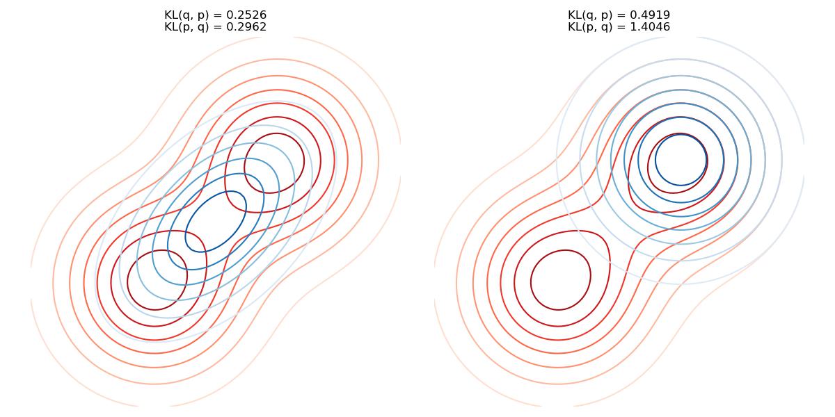
Information Projection optimizes on \(D_{KL}(q\parallel p)\)
Moment Projection optimizes on \(D_{KL}(p\parallel q)\)

First note that when \(p\approx q\), \(\log(q/p) \approx \log(p/q) \approx \log 1 = 0\) thus both projection have small values. However, consider the shape of \(\log(a/b)\), when the denominator is small, it will apply a much larger penalty. Thus, the choice of projection depends on the desired properties of wanted \(q\).

KL divergence

Source code

Evidence Lower Bound (ELBO)

Now, consider the optimization problem

\[q^* = \argmin_{\theta\in\Theta} D_{KL}(q_\theta \parallel p)\]

Note that

\[\begin{align*} D_{KL}(q_\theta \parallel p) &= E_{z\sim q_\theta} \log(\frac{q_\theta(z|x)}{p(z|x)})\\ &= E_{z\sim q_\theta} \log(\frac{q_\theta(z|x) p(x)}{p(z,x)})\\ &= E_{z\sim q_\theta} \log(\frac{q_\theta(z|x)}{p(z,x)}) + E_{z\sim q_\theta} p(x) \end{align*}\]

Since \(x\) is observed, \(E_{z\sim q_\theta} p(x)\) is fixed and independent of \(\theta\).

Thus, define the objective function s.t. minimizing \(D_{KL}(q_\theta \parallel p)\) is the same as maximizing

\[\mathcal L(\phi; x) := -E_{z\sim q_\theta} \log(\frac{q_\theta(z|x)}{p(z,x)})\]

Call \(\mathcal L(\phi)\) ELBO and note that \(-\mathcal L(\phi) + \log p(x) = D_{KL} \geq 0\implies \mathcal L(\phi)\leq \log p(x)\).

Reparameterization Trick

Now consider

\[\mathcal L(\phi; x) := -E_{z\sim q_\theta} \log(\frac{q_\theta(z|x)}{p(z,x)}) = E_{z\sim q_\theta} (\log p(x,z)-\log q_\theta(z))\]

and we are optimizing the function by

\[\nabla_\phi \mathcal L = \nabla_\phi E_{z\sim q_\theta} (\log p(x,z)-\log q_\theta(z))\]

However, this causes a problem that the expection \(E_{z\sim q_\theta}\) depends on \(q_\theta\), thus we cannot put \(\nabla_\theta\) into the expectation.

Thus, we need to reparameterize the expectation distribution, so that expectation does not depend on \(\phi\). The idea is that we use another random variable \(\epsilon\) from a fixed distribution \(p(\epsilon)\), eg. \(\text{Unif}(0,1)\) or \(N(0,1)\). Then, take some translation function \(T(\epsilon, \phi)\) s.t. \(z =T(\epsilon, \phi) \sim q_\theta(z)\). Thus, we reparameterized the expectation as

\[\begin{align*} \nabla_\phi \mathcal L &= \nabla_\phi E_{z\sim q_\theta} (\log p(x,z)-\log q_\theta(z))\\ &= \nabla_\phi E_{\epsilon\sim p(\epsilon)} (\log p(x,T(\epsilon, \phi))-\log q_\theta(T(\epsilon, \phi)))\\ &= E_{\epsilon\sim p(\epsilon)} \nabla_\phi(\log p(x,T(\epsilon, \phi))-\log q_\theta(T(\epsilon, \phi))) \end{align*}\]

Stochasitc Variational Infernce

Look at \(\nabla_\phi \mathcal L = E_{\epsilon\sim p(\epsilon)} \nabla_\phi(\log p(x,T(\epsilon, \phi))-\log q_\theta(T(\epsilon, \phi)))\), it is very similar to the gradient descent problem in neural networks. Thus, similar to SGD, we can do SVI which, at each optimization step, takes a mini-batch to estimate the sample expectation as

\[\hat E_{\epsilon\sim p(\epsilon)} \nabla_\phi (\cdots) \approx m^{-1}\sum_{i=1}^m \nabla_\theta \log(\cdots)\]